Calling DMRs with modality#
This notebooks illustrates how modality can call DMRs (differentially methylated regions). The code looks for specific group differences (e.g. healthy versus control, or sex). A brief outline of the code is described below:
We divide genome in smaller regions. Two options are available:
tiles of fixed length (e.g. 2kb)
segmentation based, in which we identify gaps in the genome where there are no CpG within a certain distance (e.g. 500bp) and divide accordingly. This is the default mode.
The contexts of each region are summed together to get the total number of methylated and unmethylated counts.
We use a logistic regression to model the methylation levels of each region. A DMR is defined as a region with a significant difference in methylation levels between two conditions. This is quantified by a p-value.
Based on this p-value, we can decide if the tile is a DMR. We also report a q-value, which is the p-value corrected using the Benjamini-Hochberg method.
from modality.dmr import call_dmrs
from modality import load_biomodal_dataset
import numpy as np
import matplotlib.pyplot as plt
import seaborn as sns
import pyranges as pr
import seaborn as sns
Load the data#
For the purposes of this demo we can use a duet +modC dataset consisting of 14 Genome in a Bottle (GIAB) samples. The data are publicly available and can be loaded using the load_biomodal_dataset() function. This will pull the dataset and load it in to our session as a ContigDataset object.
The dataset consists of 14 samples, 2 replicates of 7 cell lines. In this notebook we will look for regions of genome that are differentially methylated between two families: the Han mother-father-son trio on one hand, and the Ashkenazi mother-father-son trio on the other hand.
We merge the 2 technical replicates, and we merge the CpGs on the two strands.
ds = load_biomodal_dataset(
    name="giab",
    merge_technical_replicates=True,
    merge_cpgs=True,
    )
ds
<xarray.Dataset> Size: 12GB
Dimensions:                         (pos: 29294625, sample_id: 7)
Coordinates:
    contig                          (pos) <U20 2GB dask.array<chunksize=(40000,), meta=np.ndarray>
    ref_position                    (pos) uint32 117MB dask.array<chunksize=(40000,), meta=np.ndarray>
    strand                          (pos) <U1 117MB dask.array<chunksize=(40000,), meta=np.ndarray>
    trinucleotide_context           (pos) uint8 29MB dask.array<chunksize=(40000,), meta=np.ndarray>
  * sample_id                       (sample_id) object 56B 'HG001' ... 'HG007'
    group                           (sample_id) <U46 1kB 'CEG1530-EL01-A1200-...
    Input DNA Quantity (ng/sample)  (sample_id) int64 56B 80 80 80 80 80 80 80
    Protocol Version                (sample_id) object 56B '5-Letter v2.4' .....
    NA_id                           (sample_id) object 56B 'NA12878' ... 'NA2...
    family                          (sample_id) object 56B 'Utah' ... 'Han Ch...
    family_status                   (sample_id) object 56B 'Singleton' ... 'M...
    sex                             (sample_id) object 56B 'Female' ... 'Female'
    tech_replicate_number           (sample_id) int64 56B 1 1 1 1 1 1 1
Dimensions without coordinates: pos
Data variables:
    num_c                           (pos, sample_id) uint64 2GB dask.array<chunksize=(40000, 1), meta=np.ndarray>
    num_modc                        (pos, sample_id) uint64 2GB dask.array<chunksize=(40000, 1), meta=np.ndarray>
    num_n                           (pos, sample_id) uint64 2GB dask.array<chunksize=(40000, 1), meta=np.ndarray>
    num_other                       (pos, sample_id) uint64 2GB dask.array<chunksize=(40000, 1), meta=np.ndarray>
    num_total                       (pos, sample_id) uint64 2GB dask.array<chunksize=(40000, 1), meta=np.ndarray>
    num_total_c                     (pos, sample_id) uint64 2GB dask.array<chunksize=(40000, 1), meta=np.ndarray>
Attributes: (100/206)
    context:                     CG
    context_encoding:            {'0': 'AAA', '1': 'AAC', '10': 'AGA', '100':...
    contigs:                     ['chr1', 'chr2', 'chr3', 'chr4', 'chr5', 'ch...
    coordinate_basis:            0
    description:                 A +modC dataset of human Genome in a bottle ...
    fasta_path:                  GRCh38Decoy.fa
    grouped_on:                  giab_id
    input_path:                  ['CEG1530-EL01-A1200-001.genome.GRCh38Decoy_...
    quant_subtype:               modC
    ref_name:                    GRCh38Decoy
    sample_ids:                  ['CEG1530-EL01-A1200-001', 'CEG1530-EL01-A12...
    slice_chr1:                  slice(0, 2375159, 1)
    slice_chr10:                 slice(14996202, 16385180, 1)
    slice_chr11:                 slice(16385180, 17718294, 1)
    slice_chr11_KI270721v1_ran:  slice(29173382, 29176776, 1)
    slice_chr12:                 slice(17718294, 19034262, 1)
    slice_chr13:                 slice(19034262, 19876731, 1)
    slice_chr14:                 slice(19876731, 20739159, 1)
    slice_chr14_GL000009v2_ran:  slice(29176776, 29178255, 1)
    slice_chr14_GL000194v1_ran:  slice(29183653, 29185755, 1)
    slice_chr14_GL000225v1_ran:  slice(29178255, 29182074, 1)
    slice_chr14_KI270722v1_ran:  slice(29182074, 29183653, 1)
    slice_chr14_KI270723v1_ran:  slice(29185755, 29186353, 1)
    slice_chr14_KI270724v1_ran:  slice(29186353, 29186907, 1)
    slice_chr14_KI270725v1_ran:  slice(29186907, 29188509, 1)
    slice_chr14_KI270726v1_ran:  slice(29188509, 29189025, 1)
    slice_chr15:                 slice(20739159, 21645185, 1)
    slice_chr15_KI270727v1_ran:  slice(29189025, 29192989, 1)
    slice_chr16:                 slice(21645185, 22796076, 1)
    slice_chr16_KI270728v1_ran:  slice(29192989, 29208664, 1)
    slice_chr17:                 slice(22796076, 24044404, 1)
    slice_chr17_GL000205v2_ran:  slice(29208664, 29210537, 1)
    slice_chr17_KI270729v1_ran:  slice(29210537, 29217219, 1)
    slice_chr17_KI270730v1_ran:  slice(29217219, 29219552, 1)
    slice_chr18:                 slice(24044404, 24800418, 1)
    slice_chr19:                 slice(24800418, 25857083, 1)
    slice_chr1_KI270706v1_rand:  slice(29152891, 29154480, 1)
    slice_chr1_KI270707v1_rand:  slice(29154480, 29154791, 1)
    slice_chr1_KI270708v1_rand:  slice(29154791, 29155844, 1)
    slice_chr1_KI270709v1_rand:  slice(29155844, 29157288, 1)
    slice_chr1_KI270710v1_rand:  slice(29157288, 29157505, 1)
    slice_chr1_KI270711v1_rand:  slice(29157505, 29157882, 1)
    slice_chr1_KI270712v1_rand:  slice(29157882, 29160999, 1)
    slice_chr1_KI270713v1_rand:  slice(29160999, 29161864, 1)
    slice_chr1_KI270714v1_rand:  slice(29161864, 29163019, 1)
    slice_chr2:                  slice(2375159, 4567829, 1)
    slice_chr20:                 slice(25857083, 26630560, 1)
    slice_chr21:                 slice(26630560, 27059406, 1)
    slice_chr22:                 slice(27059406, 27660298, 1)
    slice_chr22_KI270731v1_ran:  slice(29219552, 29222033, 1)
    ...                          ...
    slice_chrUn_KI270510v1:      slice(29247760, 29247775, 1)
    slice_chrUn_KI270511v1:      slice(29248979, 29249024, 1)
    slice_chrUn_KI270512v1:      slice(29247837, 29248020, 1)
    slice_chrUn_KI270515v1:      slice(29249024, 29249065, 1)
    slice_chrUn_KI270516v1:      slice(29247829, 29247837, 1)
    slice_chrUn_KI270517v1:      slice(29249104, 29249116, 1)
    slice_chrUn_KI270518v1:      slice(29247795, 29247808, 1)
    slice_chrUn_KI270519v1:      slice(29248020, 29248909, 1)
    slice_chrUn_KI270521v1:      slice(29251667, 29251743, 1)
    slice_chrUn_KI270522v1:      slice(29248909, 29248979, 1)
    slice_chrUn_KI270528v1:      slice(29249140, 29249240, 1)
    slice_chrUn_KI270529v1:      slice(29249116, 29249140, 1)
    slice_chrUn_KI270530v1:      slice(29249240, 29249275, 1)
    slice_chrUn_KI270538v1:      slice(29249353, 29250059, 1)
    slice_chrUn_KI270539v1:      slice(29249275, 29249353, 1)
    slice_chrUn_KI270544v1:      slice(29250059, 29250078, 1)
    slice_chrUn_KI270548v1:      slice(29250078, 29250103, 1)
    slice_chrUn_KI270579v1:      slice(29250198, 29250411, 1)
    slice_chrUn_KI270580v1:      slice(29250129, 29250141, 1)
    slice_chrUn_KI270581v1:      slice(29250141, 29250198, 1)
    slice_chrUn_KI270582v1:      slice(29250753, 29250816, 1)
    slice_chrUn_KI270583v1:      slice(29250103, 29250114, 1)
    slice_chrUn_KI270584v1:      slice(29250726, 29250753, 1)
    slice_chrUn_KI270587v1:      slice(29250114, 29250129, 1)
    slice_chrUn_KI270588v1:      slice(29250816, 29250857, 1)
    slice_chrUn_KI270589v1:      slice(29250411, 29250700, 1)
    slice_chrUn_KI270590v1:      slice(29250700, 29250726, 1)
    slice_chrUn_KI270591v1:      slice(29250879, 29250912, 1)
    slice_chrUn_KI270593v1:      slice(29250857, 29250879, 1)
    slice_chrUn_KI270741v1:      slice(29263727, 29265416, 1)
    slice_chrUn_KI270742v1:      slice(29288641, 29290053, 1)
    slice_chrUn_KI270743v1:      slice(29267377, 29269464, 1)
    slice_chrUn_KI270744v1:      slice(29269464, 29271450, 1)
    slice_chrUn_KI270745v1:      slice(29271450, 29272082, 1)
    slice_chrUn_KI270746v1:      slice(29272082, 29272487, 1)
    slice_chrUn_KI270747v1:      slice(29272487, 29275904, 1)
    slice_chrUn_KI270748v1:      slice(29275904, 29277399, 1)
    slice_chrUn_KI270749v1:      slice(29277399, 29278817, 1)
    slice_chrUn_KI270750v1:      slice(29278817, 29280152, 1)
    slice_chrUn_KI270751v1:      slice(29280152, 29281268, 1)
    slice_chrUn_KI270752v1:      slice(29281268, 29281503, 1)
    slice_chrUn_KI270753v1:      slice(29281503, 29282300, 1)
    slice_chrUn_KI270754v1:      slice(29282300, 29283979, 1)
    slice_chrUn_KI270755v1:      slice(29283979, 29284530, 1)
    slice_chrUn_KI270756v1:      slice(29284530, 29286560, 1)
    slice_chrUn_KI270757v1:      slice(29286560, 29286986, 1)
    slice_chrX:                  slice(27660298, 28983007, 1)
    slice_chrY:                  slice(28983007, 29152456, 1)
    slice_chrY_KI270740v1_rand:  slice(29239647, 29239942, 1)
zarr_version: 0.1Select the two families#
First, we use the select_samples method to select only the samples corresponding to the two families of interest (i.e., the families that are not from the HG001/Utah cell line).
ds = ds.select_samples([i for i in ds.sample_id.values if i != "HG001"])
ds
<xarray.Dataset> Size: 11GB
Dimensions:                         (pos: 29294625, sample_id: 6)
Coordinates:
    contig                          (pos) <U20 2GB dask.array<chunksize=(40000,), meta=np.ndarray>
    ref_position                    (pos) uint32 117MB dask.array<chunksize=(40000,), meta=np.ndarray>
    strand                          (pos) <U1 117MB dask.array<chunksize=(40000,), meta=np.ndarray>
    trinucleotide_context           (pos) uint8 29MB dask.array<chunksize=(40000,), meta=np.ndarray>
  * sample_id                       (sample_id) object 48B 'HG002' ... 'HG007'
    group                           (sample_id) <U46 1kB 'CEG1530-EL01-A1200-...
    Input DNA Quantity (ng/sample)  (sample_id) int64 48B 80 80 80 80 80 80
    Protocol Version                (sample_id) object 48B '5-Letter v2.4' .....
    NA_id                           (sample_id) object 48B 'NA24385' ... 'NA2...
    family                          (sample_id) object 48B 'Ashkenazi Jewish'...
    family_status                   (sample_id) object 48B 'Son' ... 'Mother'
    sex                             (sample_id) object 48B 'Male' ... 'Female'
    tech_replicate_number           (sample_id) int64 48B 1 1 1 1 1 1
Dimensions without coordinates: pos
Data variables:
    num_c                           (pos, sample_id) uint64 1GB dask.array<chunksize=(40000, 1), meta=np.ndarray>
    num_modc                        (pos, sample_id) uint64 1GB dask.array<chunksize=(40000, 1), meta=np.ndarray>
    num_n                           (pos, sample_id) uint64 1GB dask.array<chunksize=(40000, 1), meta=np.ndarray>
    num_other                       (pos, sample_id) uint64 1GB dask.array<chunksize=(40000, 1), meta=np.ndarray>
    num_total                       (pos, sample_id) uint64 1GB dask.array<chunksize=(40000, 1), meta=np.ndarray>
    num_total_c                     (pos, sample_id) uint64 1GB dask.array<chunksize=(40000, 1), meta=np.ndarray>
Attributes: (100/206)
    context:                     CG
    context_encoding:            {'0': 'AAA', '1': 'AAC', '10': 'AGA', '100':...
    contigs:                     ['chr1', 'chr2', 'chr3', 'chr4', 'chr5', 'ch...
    coordinate_basis:            0
    description:                 A +modC dataset of human Genome in a bottle ...
    fasta_path:                  GRCh38Decoy.fa
    grouped_on:                  giab_id
    input_path:                  ['CEG1530-EL01-A1200-001.genome.GRCh38Decoy_...
    quant_subtype:               modC
    ref_name:                    GRCh38Decoy
    sample_ids:                  ['CEG1530-EL01-A1200-001', 'CEG1530-EL01-A12...
    slice_chr1:                  slice(0, 2375159, 1)
    slice_chr10:                 slice(14996202, 16385180, 1)
    slice_chr11:                 slice(16385180, 17718294, 1)
    slice_chr11_KI270721v1_ran:  slice(29173382, 29176776, 1)
    slice_chr12:                 slice(17718294, 19034262, 1)
    slice_chr13:                 slice(19034262, 19876731, 1)
    slice_chr14:                 slice(19876731, 20739159, 1)
    slice_chr14_GL000009v2_ran:  slice(29176776, 29178255, 1)
    slice_chr14_GL000194v1_ran:  slice(29183653, 29185755, 1)
    slice_chr14_GL000225v1_ran:  slice(29178255, 29182074, 1)
    slice_chr14_KI270722v1_ran:  slice(29182074, 29183653, 1)
    slice_chr14_KI270723v1_ran:  slice(29185755, 29186353, 1)
    slice_chr14_KI270724v1_ran:  slice(29186353, 29186907, 1)
    slice_chr14_KI270725v1_ran:  slice(29186907, 29188509, 1)
    slice_chr14_KI270726v1_ran:  slice(29188509, 29189025, 1)
    slice_chr15:                 slice(20739159, 21645185, 1)
    slice_chr15_KI270727v1_ran:  slice(29189025, 29192989, 1)
    slice_chr16:                 slice(21645185, 22796076, 1)
    slice_chr16_KI270728v1_ran:  slice(29192989, 29208664, 1)
    slice_chr17:                 slice(22796076, 24044404, 1)
    slice_chr17_GL000205v2_ran:  slice(29208664, 29210537, 1)
    slice_chr17_KI270729v1_ran:  slice(29210537, 29217219, 1)
    slice_chr17_KI270730v1_ran:  slice(29217219, 29219552, 1)
    slice_chr18:                 slice(24044404, 24800418, 1)
    slice_chr19:                 slice(24800418, 25857083, 1)
    slice_chr1_KI270706v1_rand:  slice(29152891, 29154480, 1)
    slice_chr1_KI270707v1_rand:  slice(29154480, 29154791, 1)
    slice_chr1_KI270708v1_rand:  slice(29154791, 29155844, 1)
    slice_chr1_KI270709v1_rand:  slice(29155844, 29157288, 1)
    slice_chr1_KI270710v1_rand:  slice(29157288, 29157505, 1)
    slice_chr1_KI270711v1_rand:  slice(29157505, 29157882, 1)
    slice_chr1_KI270712v1_rand:  slice(29157882, 29160999, 1)
    slice_chr1_KI270713v1_rand:  slice(29160999, 29161864, 1)
    slice_chr1_KI270714v1_rand:  slice(29161864, 29163019, 1)
    slice_chr2:                  slice(2375159, 4567829, 1)
    slice_chr20:                 slice(25857083, 26630560, 1)
    slice_chr21:                 slice(26630560, 27059406, 1)
    slice_chr22:                 slice(27059406, 27660298, 1)
    slice_chr22_KI270731v1_ran:  slice(29219552, 29222033, 1)
    ...                          ...
    slice_chrUn_KI270510v1:      slice(29247760, 29247775, 1)
    slice_chrUn_KI270511v1:      slice(29248979, 29249024, 1)
    slice_chrUn_KI270512v1:      slice(29247837, 29248020, 1)
    slice_chrUn_KI270515v1:      slice(29249024, 29249065, 1)
    slice_chrUn_KI270516v1:      slice(29247829, 29247837, 1)
    slice_chrUn_KI270517v1:      slice(29249104, 29249116, 1)
    slice_chrUn_KI270518v1:      slice(29247795, 29247808, 1)
    slice_chrUn_KI270519v1:      slice(29248020, 29248909, 1)
    slice_chrUn_KI270521v1:      slice(29251667, 29251743, 1)
    slice_chrUn_KI270522v1:      slice(29248909, 29248979, 1)
    slice_chrUn_KI270528v1:      slice(29249140, 29249240, 1)
    slice_chrUn_KI270529v1:      slice(29249116, 29249140, 1)
    slice_chrUn_KI270530v1:      slice(29249240, 29249275, 1)
    slice_chrUn_KI270538v1:      slice(29249353, 29250059, 1)
    slice_chrUn_KI270539v1:      slice(29249275, 29249353, 1)
    slice_chrUn_KI270544v1:      slice(29250059, 29250078, 1)
    slice_chrUn_KI270548v1:      slice(29250078, 29250103, 1)
    slice_chrUn_KI270579v1:      slice(29250198, 29250411, 1)
    slice_chrUn_KI270580v1:      slice(29250129, 29250141, 1)
    slice_chrUn_KI270581v1:      slice(29250141, 29250198, 1)
    slice_chrUn_KI270582v1:      slice(29250753, 29250816, 1)
    slice_chrUn_KI270583v1:      slice(29250103, 29250114, 1)
    slice_chrUn_KI270584v1:      slice(29250726, 29250753, 1)
    slice_chrUn_KI270587v1:      slice(29250114, 29250129, 1)
    slice_chrUn_KI270588v1:      slice(29250816, 29250857, 1)
    slice_chrUn_KI270589v1:      slice(29250411, 29250700, 1)
    slice_chrUn_KI270590v1:      slice(29250700, 29250726, 1)
    slice_chrUn_KI270591v1:      slice(29250879, 29250912, 1)
    slice_chrUn_KI270593v1:      slice(29250857, 29250879, 1)
    slice_chrUn_KI270741v1:      slice(29263727, 29265416, 1)
    slice_chrUn_KI270742v1:      slice(29288641, 29290053, 1)
    slice_chrUn_KI270743v1:      slice(29267377, 29269464, 1)
    slice_chrUn_KI270744v1:      slice(29269464, 29271450, 1)
    slice_chrUn_KI270745v1:      slice(29271450, 29272082, 1)
    slice_chrUn_KI270746v1:      slice(29272082, 29272487, 1)
    slice_chrUn_KI270747v1:      slice(29272487, 29275904, 1)
    slice_chrUn_KI270748v1:      slice(29275904, 29277399, 1)
    slice_chrUn_KI270749v1:      slice(29277399, 29278817, 1)
    slice_chrUn_KI270750v1:      slice(29278817, 29280152, 1)
    slice_chrUn_KI270751v1:      slice(29280152, 29281268, 1)
    slice_chrUn_KI270752v1:      slice(29281268, 29281503, 1)
    slice_chrUn_KI270753v1:      slice(29281503, 29282300, 1)
    slice_chrUn_KI270754v1:      slice(29282300, 29283979, 1)
    slice_chrUn_KI270755v1:      slice(29283979, 29284530, 1)
    slice_chrUn_KI270756v1:      slice(29284530, 29286560, 1)
    slice_chrUn_KI270757v1:      slice(29286560, 29286986, 1)
    slice_chrX:                  slice(27660298, 28983007, 1)
    slice_chrY:                  slice(28983007, 29152456, 1)
    slice_chrY_KI270740v1_rand:  slice(29239647, 29239942, 1)
zarr_version: 0.1Restrict to chromosome 1#
In this notebook, we will look for DMRs on a subset of the whole genome, here chromosome 1.
substore = ds["chr1"].copy()
Filter by coverage#
It is good practice to remove sites of low coverage before calling DMRs. This can be done with the subset_bycoverage method of the ContigDataset. Here we call it with the method="mean", which removes a position if the mean coverage of all the samples at that CpG context is strictly lower than min_coverage. Other options are "all" and "any".
substore = substore.subset_bycoverage(min_coverage=5, method="mean")
Call DMRs#
Now we can call DMRs using the call_dmrs function. We need to specify the ContigDataset object we are going to use (here substore), as well as the count variables (here num_modc and num_total_c) and the condition (here we look for DMRs across two different families, so we set use family).
Finally, call_dmrs needs to know the regions where to look for DMRs.
We can create genomic ranges using the get_ranges method, which currently has three ways of creating ranges:
The default mode, which is to pre-segment the CpGs, creating a new region every time two consecutive CpGs are separated by a distance larger than
presegment_threshold(here we use the defaultpresegment_thresholdof 500bp). This determines the regions in whichmodalityis going to look for DMRs.The fixed-window approach, where you can pass an integer, for instance
window_size=2000, which will divide the genome in tiles of size 2kbpThe
bedfileoption, where you give the path to a bedfile, and the Chromosome, Start, End columns of this bedfile will be used to create the ranges
For this dataset, it takes about 1 minutes to call DMRs on chromosome 1 on a MacBook Pro M2.
Note that you don’t have to restrict to one chromosome at a time. You can use call_dmrs on your ContigDataset ds.
ranges = ds.get_ranges(presegment_threshold=500)
Now we are ready to call DMRs.
dmr_regions = call_dmrs(
    ds=substore,
    count_array_name="num_modc",
    total_counts_name="num_total_c",
    condition_array_name="family",
    ranges=ranges,
    condition_order=["Ashkenazi Jewish", "Han Chinese"],
)
The output dmr_regions is a dataframe containing the following columns:
the chromosome, start, end (zero-based) of the region
the number of contexts in the region
the mean coverage of the region
the mean methylation fraction of each group
the methylation fold change
(mean(group_2)/mean(group_1))the methylation difference
(mean(group_2)-mean(group_1))the test statistic, in our case a Wald test
the p-value associated with the significance of the coefficient of the logistic regression associated with the group
the q-value (Benjamini-Hochberg corrected p-value)
dmr_regions.head()
| Chromosome | Start | End | num_contexts | mean_coverage | mean_mod_group_1 | mean_mod_group_2 | mod_fold_change | mod_difference | test_statistic | dmr_pvalue | dmr_qvalue | |
|---|---|---|---|---|---|---|---|---|---|---|---|---|
| ranges | ||||||||||||
| 0 | chr1 | 53833 | 54649 | 4 | 79.916667 | 0.758362 | 0.717438 | 0.946036 | -0.040924 | 66.213523 | 4.046269e-16 | 1.556977e-15 |
| 1 | chr1 | 55298 | 56585 | 9 | 84.481481 | 0.129713 | 0.402253 | 3.101088 | 0.272539 | 14.615858 | 1.318008e-04 | 2.071451e-04 |
| 2 | chr1 | 59275 | 63967 | 33 | 80.025253 | 0.369430 | 0.637943 | 1.726832 | 0.268513 | 149.556228 | 2.167498e-34 | 2.868991e-33 |
| 3 | chr1 | 64494 | 65166 | 3 | 81.833333 | 0.331799 | 0.415009 | 1.250784 | 0.083210 | 5.410776 | 2.001282e-02 | 2.562285e-02 |
| 4 | chr1 | 66899 | 67509 | 4 | 62.083333 | 0.239915 | 0.682001 | 2.842678 | 0.442086 | 0.785096 | 3.755870e-01 | 4.094675e-01 |
It is also useful to associate a slice in the format “Chromosome:Start-End” to the dataframe, since our ContigDataset object can be sliced using such string. This will come in handy later on in this notebook when we plot DMRs.
dmr_regions["Slice"] = dmr_regions.apply(
    lambda row: f"{row['Chromosome']}:{row['Start']}-{row['End']}", axis=1
)
dmr_regions.head()
| Chromosome | Start | End | num_contexts | mean_coverage | mean_mod_group_1 | mean_mod_group_2 | mod_fold_change | mod_difference | test_statistic | dmr_pvalue | dmr_qvalue | Slice | |
|---|---|---|---|---|---|---|---|---|---|---|---|---|---|
| ranges | |||||||||||||
| 0 | chr1 | 53833 | 54649 | 4 | 79.916667 | 0.758362 | 0.717438 | 0.946036 | -0.040924 | 66.213523 | 4.046269e-16 | 1.556977e-15 | chr1:53833-54649 |
| 1 | chr1 | 55298 | 56585 | 9 | 84.481481 | 0.129713 | 0.402253 | 3.101088 | 0.272539 | 14.615858 | 1.318008e-04 | 2.071451e-04 | chr1:55298-56585 |
| 2 | chr1 | 59275 | 63967 | 33 | 80.025253 | 0.369430 | 0.637943 | 1.726832 | 0.268513 | 149.556228 | 2.167498e-34 | 2.868991e-33 | chr1:59275-63967 |
| 3 | chr1 | 64494 | 65166 | 3 | 81.833333 | 0.331799 | 0.415009 | 1.250784 | 0.083210 | 5.410776 | 2.001282e-02 | 2.562285e-02 | chr1:64494-65166 |
| 4 | chr1 | 66899 | 67509 | 4 | 62.083333 | 0.239915 | 0.682001 | 2.842678 | 0.442086 | 0.785096 | 3.755870e-01 | 4.094675e-01 | chr1:66899-67509 |
Differentially Methylated Cytosines#
Instead of calling DMRs, you may be interested to know if your individual cytosines are differentially methyated or not (so called DMC’s).
In principle you could call DMCs genome-wide, but in practice it involves running one logistic regression per context. This task is time and memory intensive, and is not recommended. Instead, we can focus a small region of interest, for instance a gene or an enhancer, and look at differentially methylated contexts for this region only.
Let’s look at the GBA1 gene, associated with Gaucher disease, a genetic disease particularly common in the Ashkenazi population. The gene is on the negative strand of chr1, between positions 155234451 and 155244698 (human reference hg38). We can select this particular region in our dataset by using a slice string formatted as “Chromosome:Start-End”. So for our particular gene, we would do:
ds["chr1:155_234_451-155_244_698"]
<xarray.Dataset> Size: 75kB
Dimensions:                         (pos: 196, sample_id: 6)
Coordinates:
    contig                          (pos) <U20 16kB dask.array<chunksize=(196,), meta=np.ndarray>
    ref_position                    (pos) uint32 784B dask.array<chunksize=(196,), meta=np.ndarray>
    strand                          (pos) <U1 784B dask.array<chunksize=(196,), meta=np.ndarray>
    trinucleotide_context           (pos) uint8 196B dask.array<chunksize=(196,), meta=np.ndarray>
  * sample_id                       (sample_id) object 48B 'HG002' ... 'HG007'
    group                           (sample_id) <U46 1kB 'CEG1530-EL01-A1200-...
    Input DNA Quantity (ng/sample)  (sample_id) int64 48B 80 80 80 80 80 80
    Protocol Version                (sample_id) object 48B '5-Letter v2.4' .....
    NA_id                           (sample_id) object 48B 'NA24385' ... 'NA2...
    family                          (sample_id) object 48B 'Ashkenazi Jewish'...
    family_status                   (sample_id) object 48B 'Son' ... 'Mother'
    sex                             (sample_id) object 48B 'Male' ... 'Female'
    tech_replicate_number           (sample_id) int64 48B 1 1 1 1 1 1
Dimensions without coordinates: pos
Data variables:
    num_c                           (pos, sample_id) uint64 9kB dask.array<chunksize=(196, 1), meta=np.ndarray>
    num_modc                        (pos, sample_id) uint64 9kB dask.array<chunksize=(196, 1), meta=np.ndarray>
    num_n                           (pos, sample_id) uint64 9kB dask.array<chunksize=(196, 1), meta=np.ndarray>
    num_other                       (pos, sample_id) uint64 9kB dask.array<chunksize=(196, 1), meta=np.ndarray>
    num_total                       (pos, sample_id) uint64 9kB dask.array<chunksize=(196, 1), meta=np.ndarray>
    num_total_c                     (pos, sample_id) uint64 9kB dask.array<chunksize=(196, 1), meta=np.ndarray>
Attributes:
    context:           CG
    context_encoding:  {'0': 'AAA', '1': 'AAC', '10': 'AGA', '100': 'TAA', '1...
    contigs:           ['chr1']
    coordinate_basis:  0
    description:       A +modC dataset of human Genome in a bottle (GIAB) sam...
    fasta_path:        GRCh38Decoy.fa
    grouped_on:        giab_id
    input_path:        ['CEG1530-EL01-A1200-001.genome.GRCh38Decoy_primary_as...
    quant_subtype:     modC
    ref_name:          GRCh38Decoy
    sample_ids:        ['CEG1530-EL01-A1200-001', 'CEG1530-EL01-A1200-004', '...
    zarr_version:      0.1
slice_chr1: slice(0, 196, 1)Let’s look at DMCs in this gene. In order to achieve this, we run the get_ranges method with the window_size=1 parameter. This creates ranges of size 1bp, so each context becomes its own genomic range on which we can call differential methylation.
Note: You probably want to avoid running get_ranges(window_size=1) on a ContigDataset containing your entire genome, otherwise it will create a huge dataframe!
ranges_cpgs = ds["chr1:155_234_451-155_244_698"].get_ranges(window_size=1)
dmc_calls = call_dmrs(
    ds=ds["chr1:155_234_451-155_244_698"],
    count_array_name="num_modc",
    total_counts_name="num_total_c",
    condition_array_name="family",
    condition_order=["Ashkenazi Jewish", "Han Chinese"],
    ranges=ranges_cpgs,
)
Let’s remove positions that do not contain a context, and sites of low coverage:
dmc_calls = dmc_calls[(dmc_calls.num_contexts>0) & (dmc_calls.mean_coverage>5)]
The table below shows all the contexts in the gene, ordered by the p-value associated with their level of differential methylation.
dmc_calls.sort_values("dmr_pvalue")
| Chromosome | Start | End | num_contexts | mean_coverage | mean_mod_group_1 | mean_mod_group_2 | mod_fold_change | mod_difference | test_statistic | dmr_pvalue | dmr_qvalue | |
|---|---|---|---|---|---|---|---|---|---|---|---|---|
| ranges | ||||||||||||
| 120 | chr1 | 155241670 | 155241671 | 1 | 109.166667 | 0.231689 | 0.637695 | 2.752375 | 0.406006 | 101.937739 | 5.729453e-24 | 1.122973e-21 |
| 84 | chr1 | 155239109 | 155239110 | 1 | 91.333333 | 0.521532 | 0.885283 | 1.697466 | 0.363751 | 75.437030 | 3.772482e-18 | 3.697032e-16 |
| 134 | chr1 | 155243497 | 155243498 | 1 | 103.000000 | 0.422224 | 0.738224 | 1.748419 | 0.316000 | 67.912718 | 1.708953e-16 | 1.116516e-14 |
| 125 | chr1 | 155242045 | 155242046 | 1 | 111.666667 | 0.680953 | 0.928819 | 1.363999 | 0.247866 | 56.317558 | 6.166232e-14 | 3.021454e-12 |
| 64 | chr1 | 155237947 | 155237948 | 1 | 92.000000 | 0.669137 | 0.406847 | 0.608017 | -0.262291 | 38.760004 | 4.792476e-10 | 1.878651e-08 |
| ... | ... | ... | ... | ... | ... | ... | ... | ... | ... | ... | ... | ... |
| 69 | chr1 | 155238289 | 155238290 | 1 | 62.500000 | 0.934109 | 0.930153 | 0.995765 | -0.003956 | 0.001364 | 9.705439e-01 | 1.000000e+00 |
| 166 | chr1 | 155244259 | 155244260 | 1 | 95.833333 | 0.000000 | 0.000000 | NaN | 0.000000 | 0.000862 | 9.765759e-01 | 1.000000e+00 |
| 74 | chr1 | 155238682 | 155238683 | 1 | 104.000000 | 0.887430 | 0.887847 | 1.000470 | 0.000417 | 0.000854 | 9.766926e-01 | 1.000000e+00 |
| 27 | chr1 | 155235813 | 155235814 | 1 | 97.833333 | 0.971431 | 0.973137 | 1.001757 | 0.001707 | 0.000584 | 9.807192e-01 | 1.000000e+00 |
| 103 | chr1 | 155240047 | 155240048 | 1 | 78.333333 | 0.977477 | 0.977388 | 0.999909 | -0.000089 | 0.000207 | 9.885330e-01 | 1.000000e+00 |
186 rows × 12 columns
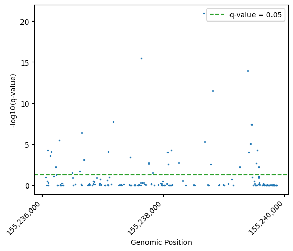
Let’s visualise the significant contexts as a Manhattan plot of their q-values:
dmc_calls["minus_log10_qvalue"] = -np.log10(dmc_calls["dmr_qvalue"])
g = sns.scatterplot(
    data=dmc_calls,
    x="Start",
    y="minus_log10_qvalue",
    edgecolor=None,
    s=5,
)

# Format axis labels
plt.xlabel("Genomic Position")
plt.ylabel("-log10(q-value)")
# add significance threshold line
plt.axhline(-np.log10(0.05), color='C2', linestyle='--', label="q-value = 0.05")

# Format x-axis labels
ticks = g.get_xticks()
xlabels = ["{:,.0f}".format(x) for x in ticks]
g.set_xticklabels(xlabels)
# Rotate x-axis labels
plt.xticks(rotation=45, ha='right')
# Only three ticks on x-axis
plt.locator_params(axis='x', nbins=3)
# Add legend
plt.legend()

plt.show()
Volcano plot of DMRs#
Now let’s return to our region-based calls. Let’s visualise the q-values of our DMR calls against the mean methylation difference between the two groups.
dmr_regions["dmr_qvalue"] = dmr_regions["dmr_qvalue"].replace(0, 10**-300)
dmr_regions["-log10 dmr_qvalue"] = -np.log10(dmr_regions["dmr_qvalue"])
g = sns.scatterplot(
    x="mod_difference",
    y="-log10 dmr_qvalue",
    data=dmr_regions,
    edgecolor=None,
    s=5,
)
g.set_xlim(-1, 1)
g.axvline(0, color="black", linewidth=0.5)
g.axvline(np.log2(1./2), color="black", linewidth=0.5, linestyle="--")
g.axvline(np.log2(2.), color="black", linewidth=0.5, linestyle="--")
<matplotlib.lines.Line2D at 0x35eeb3d90>
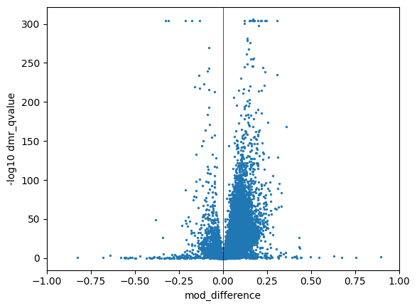
The solid black line marks the transition from hypo to hyper methylated DMRs. Hence the right-hand side of that line indicate DMRs where the Ashkenazi family is less methylated on average than the Han family.
A closer look at some DMRs#
Let’s look at regions with low q-values, high number of CpGs, and significant methylation difference. These should be our strong DMR calls.
dmrs = dmr_regions.query(
    "dmr_qvalue < 0.01 & num_contexts > 10 & (mod_difference < -0.05 | mod_difference > 0.05)"
).reset_index(drop=True)
dmrs = dmrs.sort_values("dmr_pvalue")
dmrs
| Chromosome | Start | End | num_contexts | mean_coverage | mean_mod_group_1 | mean_mod_group_2 | mod_fold_change | mod_difference | test_statistic | dmr_pvalue | dmr_qvalue | Slice | -log10 dmr_qvalue | |
|---|---|---|---|---|---|---|---|---|---|---|---|---|---|---|
| 18266 | chr1 | 244280325 | 244284050 | 63 | 96.058201 | 0.678481 | 0.849162 | 1.251563 | 0.170681 | 1424.550130 | 9.720008e-312 | 6.323545e-307 | chr1:244280325-244284050 | 306.199039 |
| 208 | chr1 | 23030631 | 23034399 | 35 | 106.819048 | 0.550659 | 0.788879 | 1.432610 | 0.238220 | 1415.936394 | 7.234870e-310 | 2.353395e-305 | chr1:23030631-23034399 | 304.628305 |
| 15086 | chr1 | 161453177 | 161458091 | 98 | 87.539116 | 0.671106 | 0.362645 | 0.540369 | -0.308461 | 4601.361013 | 2.225074e-308 | 6.893173e-305 | chr1:161453177-161458091 | 304.161581 |
| 14538 | chr1 | 143324426 | 143328909 | 128 | 36.014323 | 0.758380 | 0.933990 | 1.231560 | 0.175610 | 2026.852295 | 2.225074e-308 | 6.893173e-305 | chr1:143324426-143328909 | 304.161581 |
| 14742 | chr1 | 151131851 | 151135912 | 198 | 74.213805 | 0.766691 | 0.890421 | 1.161383 | 0.123731 | 2386.234096 | 2.225074e-308 | 6.893173e-305 | chr1:151131851-151135912 | 304.161581 |
| ... | ... | ... | ... | ... | ... | ... | ... | ... | ... | ... | ... | ... | ... | ... |
| 14232 | chr1 | 121790329 | 121795233 | 18 | 27.879630 | 0.728443 | 0.257108 | 0.352956 | -0.471335 | 8.784416 | 3.038148e-03 | 4.219293e-03 | chr1:121790329-121795233 | 2.374760 |
| 7661 | chr1 | 196779217 | 196780281 | 14 | 83.464286 | 0.571536 | 0.820029 | 1.434782 | 0.248493 | 8.585476 | 3.388547e-03 | 4.684817e-03 | chr1:196779217-196780281 | 2.329307 |
| 14540 | chr1 | 143362435 | 143367381 | 15 | 21.700000 | 0.382756 | 0.449847 | 1.175286 | 0.067092 | 8.411658 | 3.728225e-03 | 5.133786e-03 | chr1:143362435-143367381 | 2.289562 |
| 76 | chr1 | 13021960 | 13025168 | 14 | 26.619048 | 0.310078 | 0.368879 | 1.189635 | 0.058802 | 8.183784 | 4.226650e-03 | 5.788178e-03 | chr1:13021960-13025168 | 2.237458 |
| 15956 | chr1 | 196808710 | 196811438 | 39 | 68.854701 | 0.443629 | 0.638864 | 1.440085 | 0.195235 | 8.146253 | 4.315023e-03 | 5.902490e-03 | chr1:196808710-196811438 | 2.228965 |
18523 rows × 14 columns
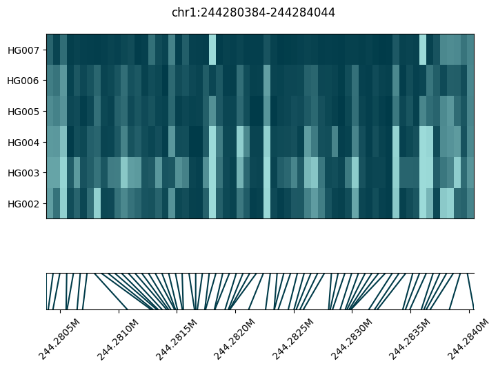
We can use the plot_methylation_tile method of the ContigDataset to plot visualise the DMRs.
In the two examples below, we can see tiles where the methylation is different between HG002, HG003, HG004 (the Ashkenazi trio) on one hand and HG005, HG006, HG007 (the Han trio) on the other hand. Each patch of color is a CpG. The dark patches correspond to CpGs with high methyation fraction, while the light patches correpond to a low methylation fraction. Grey patches (if any) are CpGs with low coverage. For each panel, the bottom plot is a locator which shows the genomic location of each CpG.
fig = substore[dmrs["Slice"].iloc[0]].plot_methylation_tile(
    numerator="num_modc",
    denominator="num_total_c",
    min_coverage=5,
)
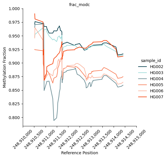
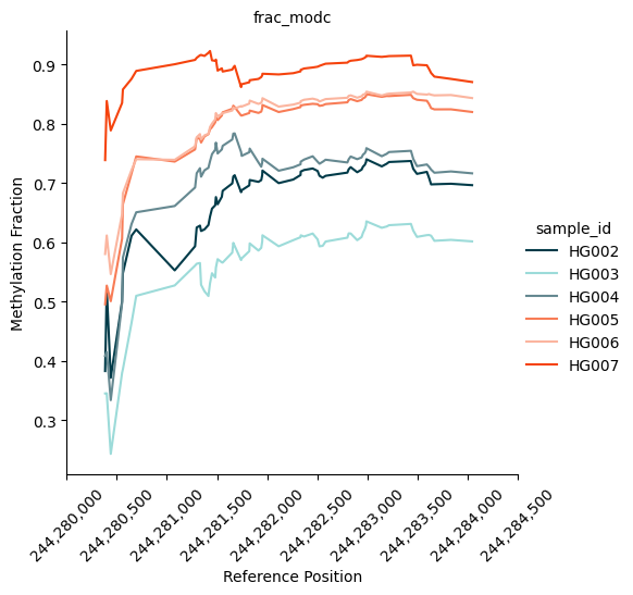
We can also plot the methylation trace. It shows the methylation fraction across the region of interest. In our case, it clearly shows a distinct pattern of methylation between the Ashkenazi group (blue-ish colours) and the Han group (red-ish colours).
kwargs = {
    "palette": ["#003B49", "#9CDBD9", "#668991", "#F87C56", "#fbb59f", "#f5430d"],
}

fig = substore[dmrs["Slice"].iloc[0]].plot_methylation_trace(
    numerators=["num_modc"],
    denominator="num_total_c",
    min_coverage=5,
    **kwargs
)
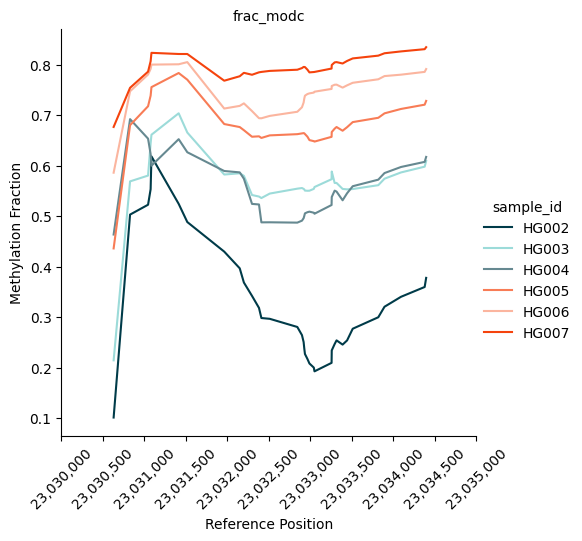
Let’s look at a second example:
fig = substore[dmrs["Slice"].iloc[1]].plot_methylation_tile(
    numerator="num_modc",
    denominator="num_total_c",
    min_coverage=5,
)
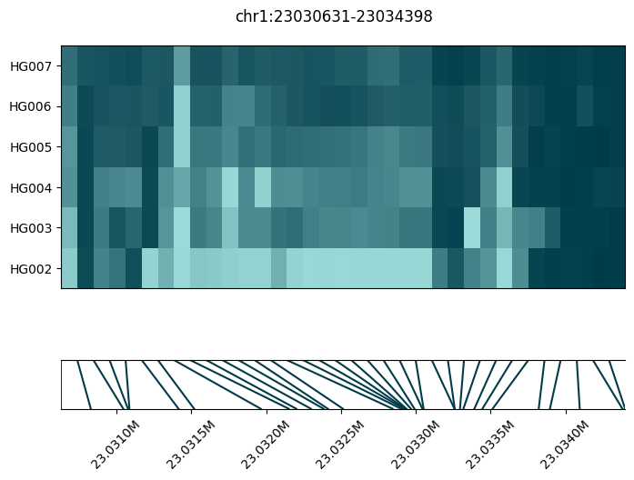
fig = substore[dmrs["Slice"].iloc[1]].plot_methylation_trace(
    numerators=["num_modc"],
    denominator="num_total_c",
    min_coverage=5,
    **kwargs
)
A non-DMR example#
In this example there is not clear difference in methylation between the two family trios, hence it was correctly not called as a DMR.
fig = substore[dmr_regions["Slice"].iloc[-7]].plot_methylation_tile(
    numerator="num_modc",
    denominator="num_total_c",
    min_coverage=5,
)
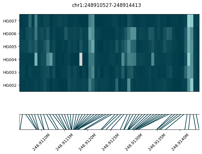
fig = substore[dmr_regions["Slice"].iloc[-7]].plot_methylation_trace(
    numerators=["num_modc"],
    denominator="num_total_c",
    min_coverage=5,
    **kwargs
)