Working with genomic ranges in modality

A common pattern when analysing methylation datasets is to perform a series of operations over specified genomic regions. modality has extensive support for working with genomic ranges via pyranges objects from the PyRanges package. In this notebook we showcase some of the working patterns and analyses that are enabled by modality when working with genomic ranges.

Load data

For the purposes of this demo we can use a duet +modC dataset of Genome in a bottle (GIAB) samples. The data are publicly available and can be loaded using the load_biomodal_dataset() function from the datasets module. This will pull the dataset and load it in to our session as a ContigDataset object.

from modality import load_biomodal_dataset

ds = load_biomodal_dataset("giab")

We will restrict to a single trio in the dataset here for the purposes of the demonstration. Once we have subset the dataset we use assign_fractions method of the ContigDataset to calculate methylation fractions.

sample_selection = ds["family"].values == "Ashkenazi Jewish"
ds = ds.sel(sample_id=sample_selection).copy()

ds.assign_fractions(
    numerators="num_modc",
    denominator="num_total_c",
    min_coverage=10,
    inplace=True,
)

Annotation via intervals

Often we will want to overlay some annotation from external sources onto the genomic regions captured in the ContigDataset. modality provides a series of built-in functions to extract genomic annotations from UCSC and GENECODE. These functions are availble via the modality.annotation module.

Using built-in functions for retrieving annotation

from modality.annotation import (
    get_cpg_islands,
    get_cpg_shores,
    get_cpg_shelves,
    get_exons,
    get_five_prime_utrs,
)

We can wrap multiple get_* functions into lists or dictionaries and then use these for downstream analysis:

contigs = [f"chr{i}" for i in range(1, 23)] + ["chrX", "chrY"]
cpg_annotations = [
    get_cpg_islands(contigs=contigs),
    get_cpg_shelves(contigs=contigs),
    get_cpg_shores(contigs=contigs),
]

For example, the first item in the cpg_annotations list here is a pyranges object of CpG islands:

cpg_islands = cpg_annotations[0]
cpg_islands

	Index	Bin	Chromosome	Start	End	Length	Cpgnum	Gcnum	Percpg	Pergc	Obsexp	Type	Ranges_ID
0	9	585	chr1	28735	29737	1002	111	731	22.2	73.0	0.85	cpg_island	0
1	10	586	chr1	135124	135563	439	30	295	13.7	67.2	0.64	cpg_island	1
2	11	586	chr1	199251	200121	870	104	643	23.9	73.9	0.89	cpg_island	2
3	12	587	chr1	368792	370063	1271	99	777	15.6	61.1	0.84	cpg_island	3
4	13	587	chr1	381172	382185	1013	84	734	16.6	72.5	0.64	cpg_island	4
...	...	...	...	...	...	...	...	...	...	...	...	...	...
27944	189	779	chrY	25464370	25464941	571	51	403	17.9	70.6	0.72	cpg_island	27944
27945	190	786	chrY	26409388	26409785	397	32	252	16.1	63.5	0.82	cpg_island	27945
27946	191	788	chrY	26627168	26627397	229	25	172	21.8	75.1	0.78	cpg_island	27946
27947	192	1020	chrY	57067645	57068034	389	36	257	18.5	66.1	0.85	cpg_island	27947
27948	193	1021	chrY	57203115	57203423	308	29	190	18.8	61.7	0.99	cpg_island	27948

27949 rows × 13 columns

Providing your own set of genomic ranges

You can also specify you own set of genomic ranges, either by loading in a file, for example a bedfile using pyranges.read_bed or building a ranges object:

import pyranges as pr

custom_ranges = pr.PyRanges(
    chromosomes=["chr1", "chr1", "chr1"],
    starts=[28735, 135124, 199251],
    ends=[29737, 135563, 200121],
)
custom_ranges

	Chromosome	Start	End
0	chr1	28735	29737
1	chr1	135124	135563
2	chr1	199251	200121

Computing over genomic ranges

Once you have a set of genomic ranges of interest we can use the reduce_byranges() method of the ContigDataset, to summarise methylation information across these ranges. In a bit more detail:

Broadly, from a set of N (chr, start, stop) intervals, applied to a dataset of C (contexts) x S (samples) we transform to an array of (start_ix, stop_ix) windows. When the set of intervals is applied, we select a function (numpy.mean or numpy.sum) that is applied to rows of the selected variable, and applied across axis 0, ie summarizing all values in the window.

Please note: currently we only support mean or sum reduction methods. We hope to address this in future releases

reduced_ds = ds.reduce_byranges(
    ranges=cpg_annotations,
    var="num_total_c",
)

This method returns an xarray.Dataset with reduced variables now computed over the ranges we specified.

reduced_ds

<xarray.Dataset> Size: 46MB
Dimensions:                         (ranges: 137687, sample_id: 6)
Coordinates:
    contig                          (ranges) <U20 11MB 'chr1' 'chr1' ... 'chrY'
    start                           (ranges) int64 1MB 28735 135124 ... 57203423
    end                             (ranges) int64 1MB 29737 135563 ... 57205423
    range_id                        (ranges) int64 1MB 0 1 2 ... 137685 137686
    num_contexts                    (ranges) int64 1MB 222 60 208 198 ... 0 0 0
    range_length                    (ranges) int64 1MB 1002 439 ... 2000 2000
    group                           (sample_id) <U22 528B 'CEG1530-EL01-A1200...
  * sample_id                       (sample_id) <U22 528B 'CEG1530-EL01-A1200...
    Input DNA Quantity (ng/sample)  (sample_id) int64 48B 80 80 80 80 80 80
    Protocol Version                (sample_id) object 48B '5-Letter v2.4' .....
    giab_id                         (sample_id) object 48B 'HG002' ... 'HG004'
    NA_id                           (sample_id) object 48B 'NA24385' ... 'NA2...
    family                          (sample_id) object 48B 'Ashkenazi Jewish'...
    family_status                   (sample_id) object 48B 'Son' ... 'Mother'
    sex                             (sample_id) object 48B 'Male' ... 'Female'
    tech_replicate_number           (sample_id) int64 48B 1 1 1 2 2 2
Dimensions without coordinates: ranges
Data variables:
    num_total_c_sum                 (ranges, sample_id) uint64 7MB dask.array<chunksize=(34422, 2), meta=np.ndarray>
    num_total_c_mean                (ranges, sample_id) float64 7MB dask.array<chunksize=(34422, 2), meta=np.ndarray>
    num_total_c_cpg_count           (ranges, sample_id) uint64 7MB dask.array<chunksize=(34422, 2), meta=np.ndarray>
    Index                           (ranges) int64 1MB 9 10 11 ... 192 193 193
    Bin                             (ranges) int64 1MB 585 586 586 ... 1021 1021
    Length                          (ranges) int64 1MB 1002 439 870 ... 308 308
    Cpgnum                          (ranges) int64 1MB 111 30 104 ... 36 29 29
    Gcnum                           (ranges) int64 1MB 731 295 643 ... 190 190
    Percpg                          (ranges) float64 1MB 22.2 13.7 ... 18.8 18.8
    Pergc                           (ranges) float64 1MB 73.0 67.2 ... 61.7 61.7
    Obsexp                          (ranges) float64 1MB 0.85 0.64 ... 0.99 0.99
    Type                            (ranges) object 1MB 'cpg_island' ... 'sho...

xarray.Dataset

• Dimensions:
  • ranges: 137687
  • sample_id: 6
• Coordinates: (16)
  • contig
    (ranges)
    <U20
    'chr1' 'chr1' ... 'chrY' 'chrY'

    array(['chr1', 'chr1', 'chr1', ..., 'chrY', 'chrY', 'chrY'], dtype='<U20')

  • start
    (ranges)
    int64
    28735 135124 ... 57201115 57203423

    array([   28735,   135124,   199251, ..., 57068034, 57201115, 57203423])

  • end
    (ranges)
    int64
    29737 135563 ... 57203115 57205423

    array([   29737,   135563,   200121, ..., 57070034, 57203115, 57205423])

  • range_id
    (ranges)
    int64
    0 1 2 3 ... 137684 137685 137686

    array([     0,      1,      2, ..., 137684, 137685, 137686])

  • num_contexts
    (ranges)
    int64
    222 60 208 198 168 ... 36 0 0 0 0

    array([222,  60, 208, ...,   0,   0,   0])

  • range_length
    (ranges)
    int64
    1002 439 870 ... 2000 2000 2000

    array([1002,  439,  870, ..., 2000, 2000, 2000])

  • group
    (sample_id)
    <U22
    'CEG1530-EL01-A1200-004' ... 'CE...

    array(['CEG1530-EL01-A1200-004', 'CEG1530-EL01-A1200-007',
           'CEG1530-EL01-A1200-010', 'CEG1532-EL01-A1200-005',
           'CEG1532-EL01-A1200-008', 'CEG1532-EL01-A1200-011'], dtype='<U22')

  • sample_id
    (sample_id)
    <U22
    'CEG1530-EL01-A1200-004' ... 'CE...

    array(['CEG1530-EL01-A1200-004', 'CEG1530-EL01-A1200-007',
           'CEG1530-EL01-A1200-010', 'CEG1532-EL01-A1200-005',
           'CEG1532-EL01-A1200-008', 'CEG1532-EL01-A1200-011'], dtype='<U22')

  • Input DNA Quantity (ng/sample)
    (sample_id)
    int64
    80 80 80 80 80 80

    array([80, 80, 80, 80, 80, 80])

  • Protocol Version
    (sample_id)
    object
    '5-Letter v2.4' ... '5-Letter v2.4'

    array(['5-Letter v2.4', '5-Letter v2.4', '5-Letter v2.4', '5-Letter v2.4',
           '5-Letter v2.4', '5-Letter v2.4'], dtype=object)

  • giab_id
    (sample_id)
    object
    'HG002' 'HG003' ... 'HG003' 'HG004'

    array(['HG002', 'HG003', 'HG004', 'HG002', 'HG003', 'HG004'], dtype=object)

  • NA_id
    (sample_id)
    object
    'NA24385' 'NA24149' ... 'NA24143'

    array(['NA24385', 'NA24149', 'NA24143', 'NA24385', 'NA24149', 'NA24143'],
          dtype=object)

  • family
    (sample_id)
    object
    'Ashkenazi Jewish' ... 'Ashkenaz...

    array(['Ashkenazi Jewish', 'Ashkenazi Jewish', 'Ashkenazi Jewish',
           'Ashkenazi Jewish', 'Ashkenazi Jewish', 'Ashkenazi Jewish'],
          dtype=object)

  • family_status
    (sample_id)
    object
    'Son' 'Father' ... 'Mother'

    array(['Son', 'Father', 'Mother', 'Son', 'Father', 'Mother'], dtype=object)

  • sex
    (sample_id)
    object
    'Male' 'Male' ... 'Male' 'Female'

    array(['Male', 'Male', 'Female', 'Male', 'Male', 'Female'], dtype=object)

  • tech_replicate_number
    (sample_id)
    int64
    1 1 1 2 2 2

    array([1, 1, 1, 2, 2, 2])

• Data variables: (12)
  • num_total_c_sum
    (ranges, sample_id)
    uint64
    dask.array<chunksize=(34422, 2), meta=np.ndarray>

    Array Chunk Bytes 6.30 MiB 537.84 kiB Shape (137687, 6) (34422, 2) Dask graph 12 chunks in 2 graph layers Data type uint64 numpy.ndarray

  • num_total_c_mean
    (ranges, sample_id)
    float64
    dask.array<chunksize=(34422, 2), meta=np.ndarray>

    Array Chunk Bytes 6.30 MiB 537.84 kiB Shape (137687, 6) (34422, 2) Dask graph 12 chunks in 8 graph layers Data type float64 numpy.ndarray

  • num_total_c_cpg_count
    (ranges, sample_id)
    uint64
    dask.array<chunksize=(34422, 2), meta=np.ndarray>

    Array Chunk Bytes 6.30 MiB 537.84 kiB Shape (137687, 6) (34422, 2) Dask graph 12 chunks in 2 graph layers Data type uint64 numpy.ndarray

  • Index
    (ranges)
    int64
    9 10 11 12 13 ... 192 192 193 193

    array([  9,  10,  11, ..., 192, 193, 193])

  • Bin
    (ranges)
    int64
    585 586 586 587 ... 1020 1021 1021

    array([ 585,  586,  586, ..., 1020, 1021, 1021])

  • Length
    (ranges)
    int64
    1002 439 870 1271 ... 389 308 308

    array([1002,  439,  870, ...,  389,  308,  308])

  • Cpgnum
    (ranges)
    int64
    111 30 104 99 84 ... 25 36 36 29 29

    array([111,  30, 104, ...,  36,  29,  29])

  • Gcnum
    (ranges)
    int64
    731 295 643 777 ... 257 257 190 190

    array([731, 295, 643, ..., 257, 190, 190])

  • Percpg
    (ranges)
    float64
    22.2 13.7 23.9 ... 18.5 18.8 18.8

    array([22.2, 13.7, 23.9, ..., 18.5, 18.8, 18.8])

  • Pergc
    (ranges)
    float64
    73.0 67.2 73.9 ... 66.1 61.7 61.7

    array([73. , 67.2, 73.9, ..., 66.1, 61.7, 61.7])

  • Obsexp
    (ranges)
    float64
    0.85 0.64 0.89 ... 0.85 0.99 0.99

    array([0.85, 0.64, 0.89, ..., 0.85, 0.99, 0.99])

  • Type
    (ranges)
    object
    'cpg_island' ... 'shores'

    array(['cpg_island', 'cpg_island', 'cpg_island', ..., 'shores', 'shores',
           'shores'], dtype=object)

• Indexes: (1)
  • sample_id
    PandasIndex

    PandasIndex(Index(['CEG1530-EL01-A1200-004', 'CEG1530-EL01-A1200-007',
           'CEG1530-EL01-A1200-010', 'CEG1532-EL01-A1200-005',
           'CEG1532-EL01-A1200-008', 'CEG1532-EL01-A1200-011'],
          dtype='object', name='sample_id'))

• Attributes: (0)

Because we have now substantially reduced the size of the dataset by performing a series of range-based reductions we can now seemlessly integrate with other standard analysis packages such as pandas.

Please Note: This transformation should only be performed when you have used modality to subset or reduce your dataset - transforming to a pandas.DataFrame before you have done so will likely crash your notebook!

reduced_ds_pandas = reduced_ds.to_dataframe()
reduced_ds_pandas

		num_total_c_sum	num_total_c_mean	num_total_c_cpg_count	contig	start	end	range_id	num_contexts	range_length	group	...	tech_replicate_number	Index	Bin	Length	Cpgnum	Gcnum	Percpg	Pergc	Obsexp	Type
ranges	sample_id
0	CEG1530-EL01-A1200-004	367	1.653153	222	chr1	28735	29737	0	222	1002	CEG1530-EL01-A1200-004	...	1	9	585	1002	111	731	22.2	73.0	0.85	cpg_island
	CEG1530-EL01-A1200-007	303	1.364865	222	chr1	28735	29737	0	222	1002	CEG1530-EL01-A1200-007	...	1	9	585	1002	111	731	22.2	73.0	0.85	cpg_island
	CEG1530-EL01-A1200-010	314	1.414414	222	chr1	28735	29737	0	222	1002	CEG1530-EL01-A1200-010	...	1	9	585	1002	111	731	22.2	73.0	0.85	cpg_island
	CEG1532-EL01-A1200-005	324	1.459459	222	chr1	28735	29737	0	222	1002	CEG1532-EL01-A1200-005	...	2	9	585	1002	111	731	22.2	73.0	0.85	cpg_island
	CEG1532-EL01-A1200-008	401	1.806306	222	chr1	28735	29737	0	222	1002	CEG1532-EL01-A1200-008	...	2	9	585	1002	111	731	22.2	73.0	0.85	cpg_island
...	...	...	...	...	...	...	...	...	...	...	...	...	...	...	...	...	...	...	...	...	...	...
137686	CEG1530-EL01-A1200-007	0	NaN	0	chrY	57203423	57205423	137686	0	2000	CEG1530-EL01-A1200-007	...	1	193	1021	308	29	190	18.8	61.7	0.99	shores
	CEG1530-EL01-A1200-010	0	NaN	0	chrY	57203423	57205423	137686	0	2000	CEG1530-EL01-A1200-010	...	1	193	1021	308	29	190	18.8	61.7	0.99	shores
	CEG1532-EL01-A1200-005	0	NaN	0	chrY	57203423	57205423	137686	0	2000	CEG1532-EL01-A1200-005	...	2	193	1021	308	29	190	18.8	61.7	0.99	shores
	CEG1532-EL01-A1200-008	0	NaN	0	chrY	57203423	57205423	137686	0	2000	CEG1532-EL01-A1200-008	...	2	193	1021	308	29	190	18.8	61.7	0.99	shores
	CEG1532-EL01-A1200-011	0	NaN	0	chrY	57203423	57205423	137686	0	2000	CEG1532-EL01-A1200-011	...	2	193	1021	308	29	190	18.8	61.7	0.99	shores

826122 rows × 27 columns

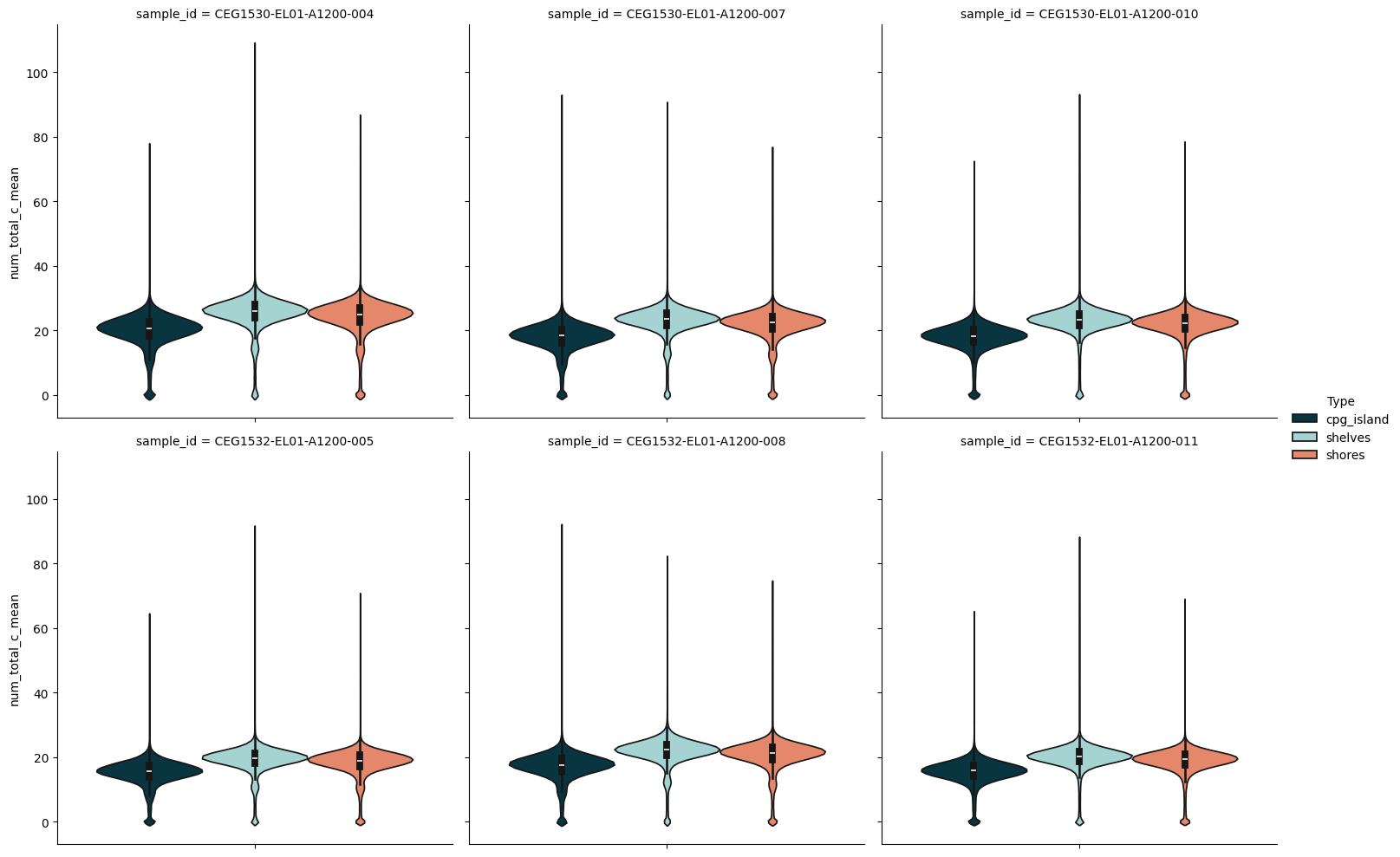
Plotting features from a reduced dataset

Having provided a set of genomic ranges of interest and then computing methylation information across these ranges and returning a new reduced dataset we can use some of modality's plotting functions to visualise the results. Below we make use of catplot and lmplot from the modality.analysis module.

from modality.analysis import catplot, lmplot

catplot(
    reduced_ds,
    col="sample_id",
    y="num_total_c_mean",
    hue="Type",
    kind="violin",
    col_wrap=3,
)

<seaborn.axisgrid.FacetGrid at 0x37b1bcb10>

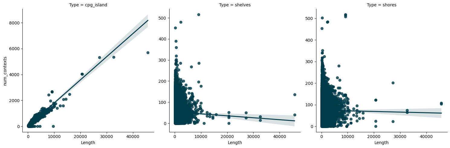
lmplot(reduced_ds, x="Length", y="num_contexts", col="Type", sharey=False)

<seaborn.axisgrid.FacetGrid at 0x38b83ef50>

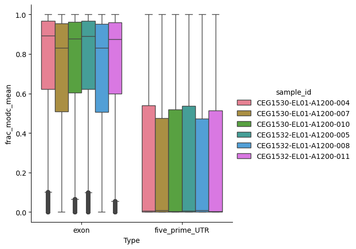
Worked example: Comparing exons to 5-prime UTRs

As another example, we can quickly reduce the dataset over exons and 5-prime UTRs and compare the methylation fractions between these two classes:

exons_range = get_exons(
    contig="chr1",
).unstrand()

five_prime_utr_range = get_five_prime_utrs(
    contig="chr1",
).unstrand()

exons_utrs_reduced = ds.reduce_byranges(
    ranges=[exons_range, five_prime_utr_range],
    var="frac_modc",
)
exons_utrs_reduced

<xarray.Dataset> Size: 31MB
Dimensions:                         (ranges: 68925, sample_id: 6)
Coordinates:
    contig                          (ranges) <U20 6MB 'chr1' 'chr1' ... 'chr1'
    start                           (ranges) int64 551kB 65418 ... 248859014
    end                             (ranges) int64 551kB 65432 ... 248859084
    range_id                        (ranges) int64 551kB 0 1 2 ... 68923 68924
    num_contexts                    (ranges) int64 551kB 0 0 36 299 ... 0 38 20
    range_length                    (ranges) int64 551kB 14 53 2548 ... 167 70
    group                           (sample_id) <U22 528B 'CEG1530-EL01-A1200...
  * sample_id                       (sample_id) <U22 528B 'CEG1530-EL01-A1200...
    Input DNA Quantity (ng/sample)  (sample_id) int64 48B 80 80 80 80 80 80
    Protocol Version                (sample_id) object 48B '5-Letter v2.4' .....
    giab_id                         (sample_id) object 48B 'HG002' ... 'HG004'
    NA_id                           (sample_id) object 48B 'NA24385' ... 'NA2...
    family                          (sample_id) object 48B 'Ashkenazi Jewish'...
    family_status                   (sample_id) object 48B 'Son' ... 'Mother'
    sex                             (sample_id) object 48B 'Male' ... 'Female'
    tech_replicate_number           (sample_id) int64 48B 1 1 1 2 2 2
Dimensions without coordinates: ranges
Data variables:
    frac_modc_sum                   (ranges, sample_id) float64 3MB dask.array<chunksize=(17232, 3), meta=np.ndarray>
    frac_modc_mean                  (ranges, sample_id) float64 3MB dask.array<chunksize=(17232, 3), meta=np.ndarray>
    frac_modc_cpg_count             (ranges, sample_id) uint64 3MB dask.array<chunksize=(17232, 3), meta=np.ndarray>
    Source                          (ranges) object 551kB 'HAVANA' ... 'HAVANA'
    Type                            (ranges) object 551kB 'exon' ... 'five_pr...
    Score                           (ranges) object 551kB '.' '.' ... '.' '.'
    Phase                           (ranges) object 551kB '.' '.' ... '.' '.'
    Id                              (ranges) object 551kB 'exon:ENST000006415...
    Parent                          (ranges) object 551kB 'ENST00000641515.2'...
    Gene_id                         (ranges) object 551kB 'ENSG00000186092.7'...
    Transcript_id                   (ranges) object 551kB 'ENST00000641515.2'...
    Gene_type                       (ranges) object 551kB 'protein_coding' .....
    Gene_name                       (ranges) object 551kB 'OR4F5' ... 'ZNF692'
    Transcript_type                 (ranges) object 551kB 'protein_coding' .....
    Transcript_name                 (ranges) object 551kB 'OR4F5-201' ... 'ZN...
    Exon_number                     (ranges) object 551kB '1' '2' ... '1' '1'
    Exon_id                         (ranges) object 551kB 'ENSE00003812156.1'...
    Level                           (ranges) object 551kB '2' '2' ... '2' '2'
    Transcript_support_level        (ranges) object 551kB '' '' '' ... '1' '1'
    Tag                             (ranges) object 551kB 'RNA_Seq_supported_...
    Havana_transcript               (ranges) object 551kB 'OTTHUMT00000003223...
    Hgnc_id                         (ranges) object 551kB 'HGNC:14825' ... 'H...
    Ont                             (ranges) object 551kB '' '' '' ... nan nan
    Havana_gene                     (ranges) object 551kB 'OTTHUMG00000001094...
    Protein_id                      (ranges) object 551kB 'ENSP00000493376.2'...
    Ccdsid                          (ranges) object 551kB 'CCDS30547.2' ... '...

xarray.Dataset

• Dimensions:
  • ranges: 68925
  • sample_id: 6
• Coordinates: (16)
  • contig
    (ranges)
    <U20
    'chr1' 'chr1' ... 'chr1' 'chr1'

    array(['chr1', 'chr1', 'chr1', ..., 'chr1', 'chr1', 'chr1'], dtype='<U20')

  • start
    (ranges)
    int64
    65418 65519 ... 248858917 248859014

    array([    65418,     65519,     69036, ..., 248858309, 248858917,
           248859014])

  • end
    (ranges)
    int64
    65432 65572 ... 248859084 248859084

    array([    65432,     65572,     71584, ..., 248858320, 248859084,
           248859084])

  • range_id
    (ranges)
    int64
    0 1 2 3 ... 68921 68922 68923 68924

    array([    0,     1,     2, ..., 68922, 68923, 68924])

  • num_contexts
    (ranges)
    int64
    0 0 36 299 299 16 ... 10 0 0 38 20

    array([ 0,  0, 36, ...,  0, 38, 20])

  • range_length
    (ranges)
    int64
    14 53 2548 1025 ... 11 11 167 70

    array([  14,   53, 2548, ...,   11,  167,   70])

  • group
    (sample_id)
    <U22
    'CEG1530-EL01-A1200-004' ... 'CE...

    array(['CEG1530-EL01-A1200-004', 'CEG1530-EL01-A1200-007',
           'CEG1530-EL01-A1200-010', 'CEG1532-EL01-A1200-005',
           'CEG1532-EL01-A1200-008', 'CEG1532-EL01-A1200-011'], dtype='<U22')

  • sample_id
    (sample_id)
    <U22
    'CEG1530-EL01-A1200-004' ... 'CE...

    array(['CEG1530-EL01-A1200-004', 'CEG1530-EL01-A1200-007',
           'CEG1530-EL01-A1200-010', 'CEG1532-EL01-A1200-005',
           'CEG1532-EL01-A1200-008', 'CEG1532-EL01-A1200-011'], dtype='<U22')

  • Input DNA Quantity (ng/sample)
    (sample_id)
    int64
    80 80 80 80 80 80

    array([80, 80, 80, 80, 80, 80])

  • Protocol Version
    (sample_id)
    object
    '5-Letter v2.4' ... '5-Letter v2.4'

    array(['5-Letter v2.4', '5-Letter v2.4', '5-Letter v2.4', '5-Letter v2.4',
           '5-Letter v2.4', '5-Letter v2.4'], dtype=object)

  • giab_id
    (sample_id)
    object
    'HG002' 'HG003' ... 'HG003' 'HG004'

    array(['HG002', 'HG003', 'HG004', 'HG002', 'HG003', 'HG004'], dtype=object)

  • NA_id
    (sample_id)
    object
    'NA24385' 'NA24149' ... 'NA24143'

    array(['NA24385', 'NA24149', 'NA24143', 'NA24385', 'NA24149', 'NA24143'],
          dtype=object)

  • family
    (sample_id)
    object
    'Ashkenazi Jewish' ... 'Ashkenaz...

    array(['Ashkenazi Jewish', 'Ashkenazi Jewish', 'Ashkenazi Jewish',
           'Ashkenazi Jewish', 'Ashkenazi Jewish', 'Ashkenazi Jewish'],
          dtype=object)

  • family_status
    (sample_id)
    object
    'Son' 'Father' ... 'Mother'

    array(['Son', 'Father', 'Mother', 'Son', 'Father', 'Mother'], dtype=object)

  • sex
    (sample_id)
    object
    'Male' 'Male' ... 'Male' 'Female'

    array(['Male', 'Male', 'Female', 'Male', 'Male', 'Female'], dtype=object)

  • tech_replicate_number
    (sample_id)
    int64
    1 1 1 2 2 2

    array([1, 1, 1, 2, 2, 2])

• Data variables: (26)
  • frac_modc_sum
    (ranges, sample_id)
    float64
    dask.array<chunksize=(17232, 3), meta=np.ndarray>

    Array Chunk Bytes 3.16 MiB 403.88 kiB Shape (68925, 6) (17232, 3) Dask graph 8 chunks in 2 graph layers Data type float64 numpy.ndarray

  • frac_modc_mean
    (ranges, sample_id)
    float64
    dask.array<chunksize=(17232, 3), meta=np.ndarray>

    Array Chunk Bytes 3.16 MiB 403.88 kiB Shape (68925, 6) (17232, 3) Dask graph 8 chunks in 8 graph layers Data type float64 numpy.ndarray

  • frac_modc_cpg_count
    (ranges, sample_id)
    uint64
    dask.array<chunksize=(17232, 3), meta=np.ndarray>

    Array Chunk Bytes 3.16 MiB 403.88 kiB Shape (68925, 6) (17232, 3) Dask graph 8 chunks in 2 graph layers Data type uint64 numpy.ndarray

  • Source
    (ranges)
    object
    'HAVANA' 'HAVANA' ... 'HAVANA'

    array(['HAVANA', 'HAVANA', 'HAVANA', ..., 'HAVANA', 'HAVANA', 'HAVANA'],
          dtype=object)

  • Type
    (ranges)
    object
    'exon' 'exon' ... 'five_prime_UTR'

    array(['exon', 'exon', 'exon', ..., 'five_prime_UTR', 'five_prime_UTR',
           'five_prime_UTR'], dtype=object)

  • Score
    (ranges)
    object
    '.' '.' '.' '.' ... '.' '.' '.' '.'

    array(['.', '.', '.', ..., '.', '.', '.'], dtype=object)

  • Phase
    (ranges)
    object
    '.' '.' '.' '.' ... '.' '.' '.' '.'

    array(['.', '.', '.', ..., '.', '.', '.'], dtype=object)

  • Id
    (ranges)
    object
    'exon:ENST00000641515.2:1' ... '...

    array(['exon:ENST00000641515.2:1', 'exon:ENST00000641515.2:2',
           'exon:ENST00000641515.2:3', ..., 'UTR5:ENST00000366471.7',
           'UTR5:ENST00000306601.9', 'UTR5:ENST00000366471.7'], dtype=object)

  • Parent
    (ranges)
    object
    'ENST00000641515.2' ... 'ENST000...

    array(['ENST00000641515.2', 'ENST00000641515.2', 'ENST00000641515.2', ...,
           'ENST00000366471.7', 'ENST00000306601.9', 'ENST00000366471.7'],
          dtype=object)

  • Gene_id
    (ranges)
    object
    'ENSG00000186092.7' ... 'ENSG000...

    array(['ENSG00000186092.7', 'ENSG00000186092.7', 'ENSG00000186092.7', ...,
           'ENSG00000171163.16', 'ENSG00000171163.16', 'ENSG00000171163.16'],
          dtype=object)

  • Transcript_id
    (ranges)
    object
    'ENST00000641515.2' ... 'ENST000...

    array(['ENST00000641515.2', 'ENST00000641515.2', 'ENST00000641515.2', ...,
           'ENST00000366471.7', 'ENST00000306601.9', 'ENST00000366471.7'],
          dtype=object)

  • Gene_type
    (ranges)
    object
    'protein_coding' ... 'protein_co...

    array(['protein_coding', 'protein_coding', 'protein_coding', ...,
           'protein_coding', 'protein_coding', 'protein_coding'], dtype=object)

  • Gene_name
    (ranges)
    object
    'OR4F5' 'OR4F5' ... 'ZNF692'

    array(['OR4F5', 'OR4F5', 'OR4F5', ..., 'ZNF692', 'ZNF692', 'ZNF692'],
          dtype=object)

  • Transcript_type
    (ranges)
    object
    'protein_coding' ... 'protein_co...

    array(['protein_coding', 'protein_coding', 'protein_coding', ...,
           'protein_coding', 'protein_coding', 'protein_coding'], dtype=object)

  • Transcript_name
    (ranges)
    object
    'OR4F5-201' ... 'ZNF692-202'

    array(['OR4F5-201', 'OR4F5-201', 'OR4F5-201', ..., 'ZNF692-202',
           'ZNF692-201', 'ZNF692-202'], dtype=object)

  • Exon_number
    (ranges)
    object
    '1' '2' '3' '1' ... '2' '2' '1' '1'

    array(['1', '2', '3', ..., '2', '1', '1'], dtype=object)

  • Exon_id
    (ranges)
    object
    'ENSE00003812156.1' ... 'ENSE000...

    array(['ENSE00003812156.1', 'ENSE00003813641.1', 'ENSE00003813949.1', ...,
           'ENSE00003586914.1', 'ENSE00003899450.1', 'ENSE00001433276.1'],
          dtype=object)

  • Level
    (ranges)
    object
    '2' '2' '2' '2' ... '2' '2' '2' '2'

    array(['2', '2', '2', ..., '2', '2', '2'], dtype=object)

  • Transcript_support_level
    (ranges)
    object
    '' '' '' '5' ... '1' '1' '1' '1'

    array(['', '', '', ..., '1', '1', '1'], dtype=object)

  • Tag
    (ranges)
    object
    'RNA_Seq_supported_partial,basic...

    array(['RNA_Seq_supported_partial,basic,Ensembl_canonical,MANE_Select,appris_principal_1,CCDS',
           'RNA_Seq_supported_partial,basic,Ensembl_canonical,MANE_Select,appris_principal_1,CCDS',
           'RNA_Seq_supported_partial,basic,Ensembl_canonical,MANE_Select,appris_principal_1,CCDS',
           ..., 'basic,appris_alternative_2,CCDS',
           'basic,Ensembl_canonical,MANE_Select,appris_principal_2,CCDS',
           'basic,appris_alternative_2,CCDS'], dtype=object)

  • Havana_transcript
    (ranges)
    object
    'OTTHUMT00000003223.4' ... 'OTTH...

    array(['OTTHUMT00000003223.4', 'OTTHUMT00000003223.4',
           'OTTHUMT00000003223.4', ..., 'OTTHUMT00000097299.1',
           'OTTHUMT00000097298.1', 'OTTHUMT00000097299.1'], dtype=object)

  • Hgnc_id
    (ranges)
    object
    'HGNC:14825' ... 'HGNC:26049'

    array(['HGNC:14825', 'HGNC:14825', 'HGNC:14825', ..., 'HGNC:26049',
           'HGNC:26049', 'HGNC:26049'], dtype=object)

  • Ont
    (ranges)
    object
    '' '' '' '' '' ... nan nan nan nan

    array(['', '', '', ..., nan, nan, nan], dtype=object)

  • Havana_gene
    (ranges)
    object
    'OTTHUMG00000001094.4' ... 'OTTH...

    array(['OTTHUMG00000001094.4', 'OTTHUMG00000001094.4',
           'OTTHUMG00000001094.4', ..., 'OTTHUMG00000040423.3',
           'OTTHUMG00000040423.3', 'OTTHUMG00000040423.3'], dtype=object)

  • Protein_id
    (ranges)
    object
    'ENSP00000493376.2' ... 'ENSP000...

    array(['ENSP00000493376.2', 'ENSP00000493376.2', 'ENSP00000493376.2', ...,
           'ENSP00000355427.3', 'ENSP00000305483.5', 'ENSP00000355427.3'],
          dtype=object)

  • Ccdsid
    (ranges)
    object
    'CCDS30547.2' ... 'CCDS53487.1'

    array(['CCDS30547.2', 'CCDS30547.2', 'CCDS30547.2', ..., 'CCDS53487.1',
           'CCDS31127.1', 'CCDS53487.1'], dtype=object)

• Indexes: (1)
  • sample_id
    PandasIndex

    PandasIndex(Index(['CEG1530-EL01-A1200-004', 'CEG1530-EL01-A1200-007',
           'CEG1530-EL01-A1200-010', 'CEG1532-EL01-A1200-005',
           'CEG1532-EL01-A1200-008', 'CEG1532-EL01-A1200-011'],
          dtype='object', name='sample_id'))

• Attributes: (0)

catplot(
    exons_utrs_reduced,
    kind='box',
    hue='sample_id',
    y='frac_modc_mean',
    x='Type',
)

<seaborn.axisgrid.FacetGrid at 0x396e3d790>

Subsetting the dataset based on genomic ranges

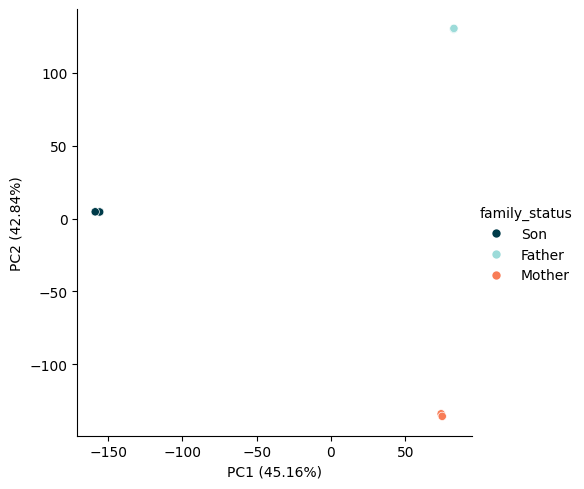
As well as reducing the dataset over a series of ranges, modality also supports subsetting the dataset, such that only CpGs that fall within a series of ranges are retained for downstream analysis. This can be very useful to restrict analyses to key regions for example. To do this we can use the subset_byranges() method of the ContigDataset. Below we use this along with a pca analysis (leveraging modality.analysis) to demonstrate this functionality and how one might use it:

from modality.analysis import run_pca, plot_pca_scatter

islands_ds = ds.subset_byranges(
    ranges=cpg_islands,
)
islands_ds

<xarray.Dataset> Size: 1GB
Dimensions:                         (pos: 4315720, sample_id: 6)
Coordinates:
    group                           (sample_id) <U22 528B dask.array<chunksize=(6,), meta=np.ndarray>
  * sample_id                       (sample_id) <U22 528B 'CEG1530-EL01-A1200...
    Input DNA Quantity (ng/sample)  (sample_id) int64 48B 80 80 80 80 80 80
    Protocol Version                (sample_id) object 48B '5-Letter v2.4' .....
    giab_id                         (sample_id) object 48B 'HG002' ... 'HG004'
    NA_id                           (sample_id) object 48B 'NA24385' ... 'NA2...
    family                          (sample_id) object 48B 'Ashkenazi Jewish'...
    family_status                   (sample_id) object 48B 'Son' ... 'Mother'
    sex                             (sample_id) object 48B 'Male' ... 'Female'
    tech_replicate_number           (sample_id) int64 48B 1 1 1 2 2 2
    contig                          (pos) <U20 345MB dask.array<chunksize=(80000,), meta=np.ndarray>
    ref_position                    (pos) uint32 17MB dask.array<chunksize=(80000,), meta=np.ndarray>
    strand                          (pos) <U2 35MB dask.array<chunksize=(80000,), meta=np.ndarray>
    trinucleotide_context           (pos) uint8 4MB dask.array<chunksize=(80000,), meta=np.ndarray>
Dimensions without coordinates: pos
Data variables:
    num_c                           (pos, sample_id) uint32 104MB dask.array<chunksize=(80000, 6), meta=np.ndarray>
    num_modc                        (pos, sample_id) uint32 104MB dask.array<chunksize=(80000, 6), meta=np.ndarray>
    num_n                           (pos, sample_id) uint32 104MB dask.array<chunksize=(80000, 6), meta=np.ndarray>
    num_other                       (pos, sample_id) uint32 104MB dask.array<chunksize=(80000, 6), meta=np.ndarray>
    num_total                       (pos, sample_id) uint32 104MB dask.array<chunksize=(80000, 6), meta=np.ndarray>
    num_total_c                     (pos, sample_id) uint32 104MB dask.array<chunksize=(80000, 6), meta=np.ndarray>
    frac_modc                       (pos, sample_id) float64 207MB dask.array<chunksize=(80000, 6), meta=np.ndarray>
Attributes:
    context:            CG
    context_encoding:   {'0': 'AAA', '1': 'AAC', '10': 'AGA', '100': 'TAA', '...
    contigs:            ['chr1', 'chr2', 'chr3', 'chr4', 'chr5', 'chr6', 'chr...
    coordinate_basis:   0
    description:        A +modC dataset of human Genome in a bottle (GIAB) sa...
    fasta_path:         GRCh38Decoy.fa
    frac_denominator:   num_total_c
    frac_min_coverage:  10
    input_path:         ['CEG1530-EL01-A1200-001.genome.GRCh38Decoy_primary_a...
    quant_subtype:      modC
    ref_name:           GRCh38Decoy
    sample_ids:         ['CEG1530-EL01-A1200-001', 'CEG1530-EL01-A1200-004', ...
    slice_chr1:         slice(0, 388278, 1)
    slice_chr10:        slice(2006948, 2207692, 1)
    slice_chr11:        slice(2207692, 2416334, 1)
    slice_chr12:        slice(2416334, 2589760, 1)
    slice_chr13:        slice(2589760, 2683988, 1)
    slice_chr14:        slice(2683988, 2814352, 1)
    slice_chr15:        slice(2814352, 2950224, 1)
    slice_chr16:        slice(2950224, 3173146, 1)
    slice_chr17:        slice(3173146, 3433468, 1)
    slice_chr18:        slice(3433468, 3523034, 1)
    slice_chr19:        slice(3523034, 3841880, 1)
    slice_chr2:         slice(388278, 671346, 1)
    slice_chr20:        slice(3841880, 3972924, 1)
    slice_chr21:        slice(3972924, 4044738, 1)
    slice_chr22:        slice(4044738, 4168048, 1)
    slice_chr3:         slice(671346, 852496, 1)
    slice_chr4:         slice(852496, 1020792, 1)
    slice_chr5:         slice(1020792, 1214570, 1)
    slice_chr6:         slice(1214570, 1404772, 1)
    slice_chr7:         slice(1404772, 1638222, 1)
    slice_chr8:         slice(1638222, 1813300, 1)
    slice_chr9:         slice(1813300, 2006948, 1)
    slice_chrX:         slice(4168048, 4307462, 1)
    slice_chrY:         slice(4307462, 4315720, 1)
    zarr_version:       0.1

xarray.Dataset

• Dimensions:
  • pos: 4315720
  • sample_id: 6
• Coordinates: (14)
  • group
    (sample_id)
    <U22
    dask.array<chunksize=(6,), meta=np.ndarray>

    Array Chunk Bytes 528 B 528 B Shape (6,) (6,) Dask graph 1 chunks in 3 graph layers Data type

  • sample_id
    (sample_id)
    <U22
    'CEG1530-EL01-A1200-004' ... 'CE...

    array(['CEG1530-EL01-A1200-004', 'CEG1530-EL01-A1200-007',
           'CEG1530-EL01-A1200-010', 'CEG1532-EL01-A1200-005',
           'CEG1532-EL01-A1200-008', 'CEG1532-EL01-A1200-011'], dtype='<U22')

  • Input DNA Quantity (ng/sample)
    (sample_id)
    int64
    80 80 80 80 80 80

    array([80, 80, 80, 80, 80, 80])

  • Protocol Version
    (sample_id)
    object
    '5-Letter v2.4' ... '5-Letter v2.4'

    array(['5-Letter v2.4', '5-Letter v2.4', '5-Letter v2.4', '5-Letter v2.4',
           '5-Letter v2.4', '5-Letter v2.4'], dtype=object)

  • giab_id
    (sample_id)
    object
    'HG002' 'HG003' ... 'HG003' 'HG004'

    array(['HG002', 'HG003', 'HG004', 'HG002', 'HG003', 'HG004'], dtype=object)

  • NA_id
    (sample_id)
    object
    'NA24385' 'NA24149' ... 'NA24143'

    array(['NA24385', 'NA24149', 'NA24143', 'NA24385', 'NA24149', 'NA24143'],
          dtype=object)

  • family
    (sample_id)
    object
    'Ashkenazi Jewish' ... 'Ashkenaz...

    array(['Ashkenazi Jewish', 'Ashkenazi Jewish', 'Ashkenazi Jewish',
           'Ashkenazi Jewish', 'Ashkenazi Jewish', 'Ashkenazi Jewish'],
          dtype=object)

  • family_status
    (sample_id)
    object
    'Son' 'Father' ... 'Mother'

    array(['Son', 'Father', 'Mother', 'Son', 'Father', 'Mother'], dtype=object)

  • sex
    (sample_id)
    object
    'Male' 'Male' ... 'Male' 'Female'

    array(['Male', 'Male', 'Female', 'Male', 'Male', 'Female'], dtype=object)

  • tech_replicate_number
    (sample_id)
    int64
    1 1 1 2 2 2

    array([1, 1, 1, 2, 2, 2])

  • contig
    (pos)
    <U20
    dask.array<chunksize=(80000,), meta=np.ndarray>

    Array Chunk Bytes 329.26 MiB 6.10 MiB Shape (4315720,) (80000,) Dask graph 54 chunks in 4 graph layers Data type

  • ref_position
    (pos)
    uint32
    dask.array<chunksize=(80000,), meta=np.ndarray>

    Array Chunk Bytes 16.46 MiB 312.50 kiB Shape (4315720,) (80000,) Dask graph 54 chunks in 4 graph layers Data type uint32 numpy.ndarray

  • strand
    (pos)
    <U2
    dask.array<chunksize=(80000,), meta=np.ndarray>

    Array Chunk Bytes 32.93 MiB 625.00 kiB Shape (4315720,) (80000,) Dask graph 54 chunks in 4 graph layers Data type

  • trinucleotide_context
    (pos)
    uint8
    dask.array<chunksize=(80000,), meta=np.ndarray>

    Array Chunk Bytes 4.12 MiB 78.12 kiB Shape (4315720,) (80000,) Dask graph 54 chunks in 4 graph layers Data type uint8 numpy.ndarray

• Data variables: (7)
  • num_c
    (pos, sample_id)
    uint32
    dask.array<chunksize=(80000, 6), meta=np.ndarray>

    Array Chunk Bytes 98.78 MiB 1.83 MiB Shape (4315720, 6) (80000, 6) Dask graph 54 chunks in 5 graph layers Data type uint32 numpy.ndarray

  • num_modc
    (pos, sample_id)
    uint32
    dask.array<chunksize=(80000, 6), meta=np.ndarray>

    Array Chunk Bytes 98.78 MiB 1.83 MiB Shape (4315720, 6) (80000, 6) Dask graph 54 chunks in 5 graph layers Data type uint32 numpy.ndarray

  • num_n
    (pos, sample_id)
    uint32
    dask.array<chunksize=(80000, 6), meta=np.ndarray>

    Array Chunk Bytes 98.78 MiB 1.83 MiB Shape (4315720, 6) (80000, 6) Dask graph 54 chunks in 5 graph layers Data type uint32 numpy.ndarray

  • num_other
    (pos, sample_id)
    uint32
    dask.array<chunksize=(80000, 6), meta=np.ndarray>

    Array Chunk Bytes 98.78 MiB 1.83 MiB Shape (4315720, 6) (80000, 6) Dask graph 54 chunks in 5 graph layers Data type uint32 numpy.ndarray

  • num_total
    (pos, sample_id)
    uint32
    dask.array<chunksize=(80000, 6), meta=np.ndarray>

    Array Chunk Bytes 98.78 MiB 1.83 MiB Shape (4315720, 6) (80000, 6) Dask graph 54 chunks in 5 graph layers Data type uint32 numpy.ndarray

  • num_total_c
    (pos, sample_id)
    uint32
    dask.array<chunksize=(80000, 6), meta=np.ndarray>

    Array Chunk Bytes 98.78 MiB 1.83 MiB Shape (4315720, 6) (80000, 6) Dask graph 54 chunks in 5 graph layers Data type uint32 numpy.ndarray

  • frac_modc
    (pos, sample_id)
    float64
    dask.array<chunksize=(80000, 6), meta=np.ndarray>

    Array Chunk Bytes 197.56 MiB 3.66 MiB Shape (4315720, 6) (80000, 6) Dask graph 54 chunks in 12 graph layers Data type float64 numpy.ndarray

• Indexes: (1)
  • sample_id
    PandasIndex

    PandasIndex(Index(['CEG1530-EL01-A1200-004', 'CEG1530-EL01-A1200-007',
           'CEG1530-EL01-A1200-010', 'CEG1532-EL01-A1200-005',
           'CEG1532-EL01-A1200-008', 'CEG1532-EL01-A1200-011'],
          dtype='object', name='sample_id'))

• Attributes: (37)

  context :

  CG

  context_encoding :

  {'0': 'AAA', '1': 'AAC', '10': 'AGA', '100': 'TAA', '101': 'TAC', '102': 'TAG', '103': 'TAN', '104': 'TAT', '105': 'TCA', '106': 'TCC', '107': 'TCG', '108': 'TCN', '109': 'TCT', '11': 'AGC', '110': 'TGA', '111': 'TGC', '112': 'TGG', '113': 'TGN', '114': 'TGT', '115': 'TNA', '116': 'TNC', '117': 'TNG', '118': 'TNN', '119': 'TNT', '12': 'AGG', '120': 'TTA', '121': 'TTC', '122': 'TTG', '123': 'TTN', '124': 'TTT', '125': 'CG', '13': 'AGN', '14': 'AGT', '15': 'ANA', '16': 'ANC', '17': 'ANG', '18': 'ANN', '19': 'ANT', '2': 'AAG', '20': 'ATA', '21': 'ATC', '22': 'ATG', '23': 'ATN', '24': 'ATT', '25': 'CAA', '255': 'unknown', '26': 'CAC', '27': 'CAG', '28': 'CAN', '29': 'CAT', '3': 'AAN', '30': 'CCA', '31': 'CCC', '32': 'CCG', '33': 'CCN', '34': 'CCT', '35': 'CGA', '36': 'CGC', '37': 'CGG', '38': 'CGN', '39': 'CGT', '4': 'AAT', '40': 'CNA', '41': 'CNC', '42': 'CNG', '43': 'CNN', '44': 'CNT', '45': 'CTA', '46': 'CTC', '47': 'CTG', '48': 'CTN', '49': 'CTT', '5': 'ACA', '50': 'GAA', '51': 'GAC', '52': 'GAG', '53': 'GAN', '54': 'GAT', '55': 'GCA', '56': 'GCC', '57': 'GCG', '58': 'GCN', '59': 'GCT', '6': 'ACC', '60': 'GGA', '61': 'GGC', '62': 'GGG', '63': 'GGN', '64': 'GGT', '65': 'GNA', '66': 'GNC', '67': 'GNG', '68': 'GNN', '69': 'GNT', '7': 'ACG', '70': 'GTA', '71': 'GTC', '72': 'GTG', '73': 'GTN', '74': 'GTT', '75': 'NAA', '76': 'NAC', '77': 'NAG', '78': 'NAN', '79': 'NAT', '8': 'ACN', '80': 'NCA', '81': 'NCC', '82': 'NCG', '83': 'NCN', '84': 'NCT', '85': 'NGA', '86': 'NGC', '87': 'NGG', '88': 'NGN', '89': 'NGT', '9': 'ACT', '90': 'NNA', '91': 'NNC', '92': 'NNG', '93': 'NNN', '94': 'NNT', '95': 'NTA', '96': 'NTC', '97': 'NTG', '98': 'NTN', '99': 'NTT'}

  contigs :

  ['chr1', 'chr2', 'chr3', 'chr4', 'chr5', 'chr6', 'chr7', 'chr8', 'chr9', 'chr10', 'chr11', 'chr12', 'chr13', 'chr14', 'chr15', 'chr16', 'chr17', 'chr18', 'chr19', 'chr20', 'chr21', 'chr22', 'chrX', 'chrY']

  coordinate_basis :

  0

  description :

  A +modC dataset of human Genome in a bottle (GIAB) samples. These data were generated by biomodal using a commercial kit. Each of the seven GIAB samples were sequenced on a single lane of a NovaSeq S4 flowcell. Two technical replicates are available for each sample.

  fasta_path :

  GRCh38Decoy.fa

  frac_denominator :

  num_total_c

  frac_min_coverage :

  10

  input_path :

  ['CEG1530-EL01-A1200-001.genome.GRCh38Decoy_primary_assembly.dedup.bam', 'CEG1530-EL01-A1200-004.genome.GRCh38Decoy_primary_assembly.dedup.bam', 'CEG1530-EL01-A1200-007.genome.GRCh38Decoy_primary_assembly.dedup.bam', 'CEG1530-EL01-A1200-010.genome.GRCh38Decoy_primary_assembly.dedup.bam', 'CEG1530-EL01-A1200-013.genome.GRCh38Decoy_primary_assembly.dedup.bam', 'CEG1530-EL01-A1200-016.genome.GRCh38Decoy_primary_assembly.dedup.bam', 'CEG1530-EL01-A1200-019.genome.GRCh38Decoy_primary_assembly.dedup.bam', 'CEG1532-EL01-A1200-002.genome.GRCh38Decoy_primary_assembly.dedup.bam', 'CEG1532-EL01-A1200-005.genome.GRCh38Decoy_primary_assembly.dedup.bam', 'CEG1532-EL01-A1200-008.genome.GRCh38Decoy_primary_assembly.dedup.bam', 'CEG1532-EL01-A1200-011.genome.GRCh38Decoy_primary_assembly.dedup.bam', 'CEG1532-EL01-A1200-015.genome.GRCh38Decoy_primary_assembly.dedup.bam', 'CEG1532-EL01-A1200-017.genome.GRCh38Decoy_primary_assembly.dedup.bam', 'CEG1532-EL01-A1200-020.genome.GRCh38Decoy_primary_assembly.dedup.bam']

  quant_subtype :

  modC

  ref_name :

  GRCh38Decoy

  sample_ids :

  ['CEG1530-EL01-A1200-001', 'CEG1530-EL01-A1200-004', 'CEG1530-EL01-A1200-007', 'CEG1530-EL01-A1200-010', 'CEG1530-EL01-A1200-013', 'CEG1530-EL01-A1200-016', 'CEG1530-EL01-A1200-019', 'CEG1532-EL01-A1200-002', 'CEG1532-EL01-A1200-005', 'CEG1532-EL01-A1200-008', 'CEG1532-EL01-A1200-011', 'CEG1532-EL01-A1200-015', 'CEG1532-EL01-A1200-017', 'CEG1532-EL01-A1200-020']

  slice_chr1 :

  slice(0, 388278, 1)

  slice_chr10 :

  slice(2006948, 2207692, 1)

  slice_chr11 :

  slice(2207692, 2416334, 1)

  slice_chr12 :

  slice(2416334, 2589760, 1)

  slice_chr13 :

  slice(2589760, 2683988, 1)

  slice_chr14 :

  slice(2683988, 2814352, 1)

  slice_chr15 :

  slice(2814352, 2950224, 1)

  slice_chr16 :

  slice(2950224, 3173146, 1)

  slice_chr17 :

  slice(3173146, 3433468, 1)

  slice_chr18 :

  slice(3433468, 3523034, 1)

  slice_chr19 :

  slice(3523034, 3841880, 1)

  slice_chr2 :

  slice(388278, 671346, 1)

  slice_chr20 :

  slice(3841880, 3972924, 1)

  slice_chr21 :

  slice(3972924, 4044738, 1)

  slice_chr22 :

  slice(4044738, 4168048, 1)

  slice_chr3 :

  slice(671346, 852496, 1)

  slice_chr4 :

  slice(852496, 1020792, 1)

  slice_chr5 :

  slice(1020792, 1214570, 1)

  slice_chr6 :

  slice(1214570, 1404772, 1)

  slice_chr7 :

  slice(1404772, 1638222, 1)

  slice_chr8 :

  slice(1638222, 1813300, 1)

  slice_chr9 :

  slice(1813300, 2006948, 1)

  slice_chrX :

  slice(4168048, 4307462, 1)

  slice_chrY :

  slice(4307462, 4315720, 1)

  zarr_version :

  0.1

pca_object, transformed_data = run_pca(
    input_array=islands_ds.frac_modc,
)

plot_pca_scatter(
    pca_object=pca_object,
    pca_result=transformed_data,
    hue=islands_ds.family_status,
)

<seaborn.axisgrid.FacetGrid at 0x39bf21f50>