Plotting methylation fractions across genomic regions#
This notebook illustrates how modality can be used to quickly and easily generate methylation trace plots - summarising methylation fractions across a genomic region of interest. This functionality offers a very rapid way to explore key genomic regions - as defined by your own research questions - and generate extensible plots. The core method provides a wrapper to seaborn.relplot allowing full customisation.
Load the data#
For the purposes of this demo we can use a duet evoC dataset of mouse ES-E14 cells. The data are publicly available and can be loaded using the load_biomodal_dataset() function. This will pull the dataset and load it in to our session as a ContigDataset object.
from modality import load_biomodal_dataset
ds = load_biomodal_dataset("esE14")
ds
<xarray.Dataset> Size: 10GB
Dimensions:                         (pos: 43816016, sample_id: 4)
Coordinates:
    contig                          (pos) <U20 4GB dask.array<chunksize=(80000,), meta=np.ndarray>
    group                           (sample_id) <U22 352B dask.array<chunksize=(4,), meta=np.ndarray>
    ref_position                    (pos) uint32 175MB dask.array<chunksize=(80000,), meta=np.ndarray>
  * sample_id                       (sample_id) <U22 352B 'CEG1485-EL01-D1115...
    strand                          (pos) <U2 351MB dask.array<chunksize=(80000,), meta=np.ndarray>
    trinucleotide_context           (pos) uint8 44MB dask.array<chunksize=(80000,), meta=np.ndarray>
    Input DNA Quantity (ng/sample)  (sample_id) int64 32B 80 80 80 80
    Protocol Version                (sample_id) object 32B '6-Letter v0.1.8' ...
    tech_replicate_number           (sample_id) int64 32B 1 2 3 4
Dimensions without coordinates: pos
Data variables:
    num_c                           (pos, sample_id) uint32 701MB dask.array<chunksize=(80000, 4), meta=np.ndarray>
    num_hmc                         (pos, sample_id) uint32 701MB dask.array<chunksize=(80000, 4), meta=np.ndarray>
    num_mc                          (pos, sample_id) uint32 701MB dask.array<chunksize=(80000, 4), meta=np.ndarray>
    num_modc                        (pos, sample_id) uint32 701MB dask.array<chunksize=(80000, 4), meta=np.ndarray>
    num_n                           (pos, sample_id) uint32 701MB dask.array<chunksize=(80000, 4), meta=np.ndarray>
    num_other                       (pos, sample_id) uint32 701MB dask.array<chunksize=(80000, 4), meta=np.ndarray>
    num_total                       (pos, sample_id) uint32 701MB dask.array<chunksize=(80000, 4), meta=np.ndarray>
    num_total_c                     (pos, sample_id) uint32 701MB dask.array<chunksize=(80000, 4), meta=np.ndarray>
Attributes:
    context:           CG
    context_encoding:  {'0': 'AAA', '1': 'AAC', '10': 'AGA', '100': 'TAA', '1...
    contigs:           ['chr1', 'chr2', 'chr3', 'chr4', 'chr5', 'chr6', 'chr7...
    coordinate_basis:  0
    fasta_path:        GRCm38p6.fa
    input_path:        ['CEG1485-EL01-D1115-001.genome.GRCm38p6_primary_assem...
    quant_subtype:     evoC
    ref_name:          GRCm38p6
    sample_ids:        ['CEG1485-EL01-D1115-001', 'CEG1485-EL01-D1115-002', '...
    slice_GL456210.1:  slice(43735674, 43738588, 1)
    slice_GL456211.1:  slice(43738588, 43742900, 1)
    slice_GL456212.1:  slice(43742900, 43745240, 1)
    slice_GL456213.1:  slice(43745240, 43746246, 1)
    slice_GL456216.1:  slice(43746246, 43748248, 1)
    slice_GL456219.1:  slice(43748248, 43750250, 1)
    slice_GL456221.1:  slice(43750250, 43753378, 1)
    slice_GL456233.1:  slice(43753378, 43756268, 1)
    slice_GL456239.1:  slice(43756268, 43756766, 1)
    slice_GL456350.1:  slice(43756766, 43761832, 1)
    slice_GL456354.1:  slice(43761832, 43764052, 1)
    slice_GL456359.1:  slice(43764052, 43764418, 1)
    slice_GL456360.1:  slice(43764418, 43764850, 1)
    slice_GL456366.1:  slice(43764850, 43765592, 1)
    slice_GL456367.1:  slice(43765592, 43766170, 1)
    slice_GL456368.1:  slice(43766170, 43766410, 1)
    slice_GL456370.1:  slice(43766410, 43767340, 1)
    slice_GL456372.1:  slice(43767340, 43767752, 1)
    slice_GL456378.1:  slice(43767752, 43768274, 1)
    slice_GL456379.1:  slice(43768274, 43769044, 1)
    slice_GL456381.1:  slice(43769044, 43769264, 1)
    slice_GL456382.1:  slice(43769264, 43769536, 1)
    slice_GL456383.1:  slice(43769536, 43770646, 1)
    slice_GL456385.1:  slice(43770646, 43771014, 1)
    slice_GL456387.1:  slice(43771014, 43771266, 1)
    slice_GL456389.1:  slice(43771266, 43772058, 1)
    slice_GL456390.1:  slice(43772058, 43772526, 1)
    slice_GL456392.1:  slice(43772526, 43773276, 1)
    slice_GL456393.1:  slice(43773276, 43774142, 1)
    slice_GL456394.1:  slice(43774142, 43774434, 1)
    slice_GL456396.1:  slice(43774434, 43775226, 1)
    slice_JH584292.1:  slice(43775226, 43775374, 1)
    slice_JH584293.1:  slice(43775374, 43780716, 1)
    slice_JH584294.1:  slice(43780716, 43785326, 1)
    slice_JH584295.1:  slice(43785326, 43785556, 1)
    slice_JH584296.1:  slice(43785556, 43787738, 1)
    slice_JH584297.1:  slice(43787738, 43789964, 1)
    slice_JH584298.1:  slice(43789964, 43792182, 1)
    slice_JH584299.1:  slice(43792182, 43803500, 1)
    slice_JH584300.1:  slice(43803500, 43805680, 1)
    slice_JH584301.1:  slice(43805680, 43808544, 1)
    slice_JH584302.1:  slice(43808544, 43810446, 1)
    slice_JH584303.1:  slice(43810446, 43812474, 1)
    slice_JH584304.1:  slice(43812474, 43816016, 1)
    slice_chr1:        slice(0, 2955122, 1)
    slice_chr10:       slice(22942856, 25156266, 1)
    slice_chr11:       slice(25156266, 27483352, 1)
    slice_chr12:       slice(27483352, 29396382, 1)
    slice_chr13:       slice(29396382, 31363950, 1)
    slice_chr14:       slice(31363950, 33246688, 1)
    slice_chr15:       slice(33246688, 34988556, 1)
    slice_chr16:       slice(34988556, 36499138, 1)
    slice_chr17:       slice(36499138, 38208052, 1)
    slice_chr18:       slice(38208052, 39651134, 1)
    slice_chr19:       slice(39651134, 40767246, 1)
    slice_chr2:        slice(2955122, 5997996, 1)
    slice_chr3:        slice(5997996, 8380428, 1)
    slice_chr4:        slice(8380428, 11046376, 1)
    slice_chr5:        slice(11046376, 13751626, 1)
    slice_chr6:        slice(13751626, 16083622, 1)
    slice_chr7:        slice(16083622, 18533500, 1)
    slice_chr8:        slice(18533500, 20801442, 1)
    slice_chr9:        slice(20801442, 22942856, 1)
    slice_chrM:        slice(43735100, 43735674, 1)
    slice_chrX:        slice(40767246, 42706184, 1)
    slice_chrY:        slice(42706184, 43735100, 1)
    zarr_version:      0.1
description: An evoC dataset of mouse ES-E14 cells, data contains 4...Extract specific genomic regions#
We can use the slice functionality of the ContigDataset to extract a specific genomic region prior to plotting the methylation trace. Below we specify three seperate data slices to show some methylation trace plots.
# Specify some genomic regions for downstream plotting - specified as chr:start-end
sliced_data= {
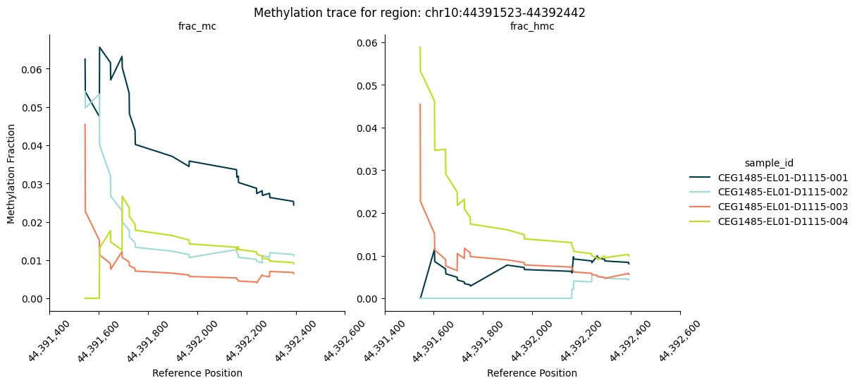
"slice_1": ds["chr10:44391523-44392442"],
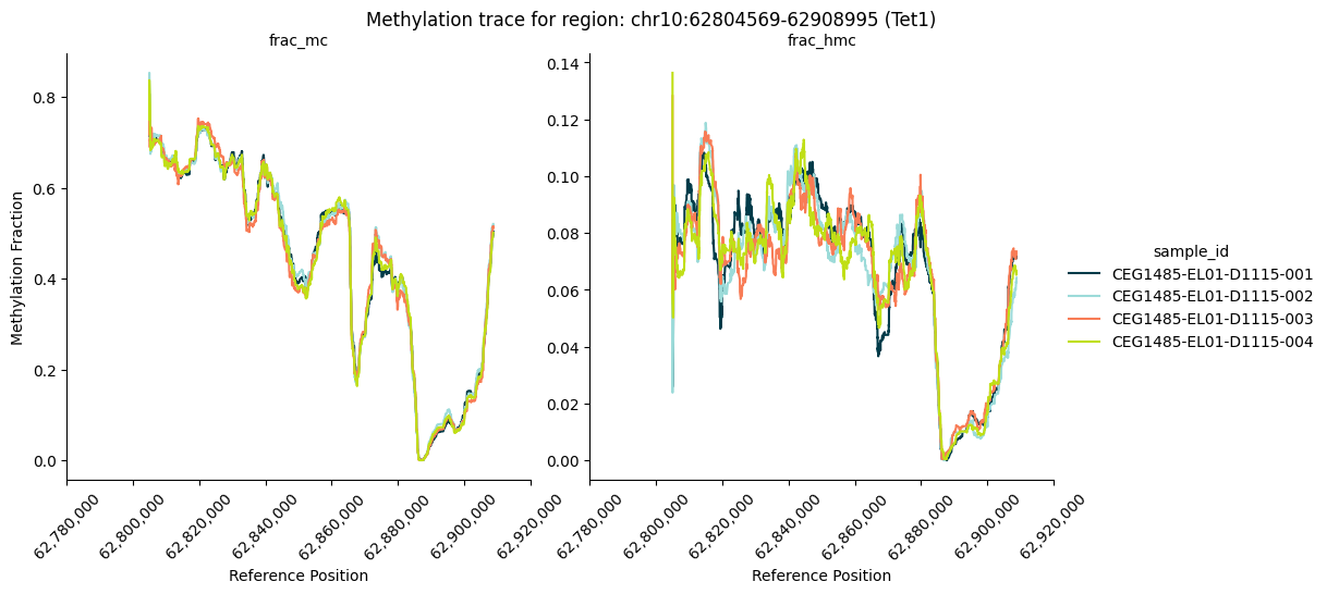
"tet1_slice": ds["chr10:62804569-62908995"],
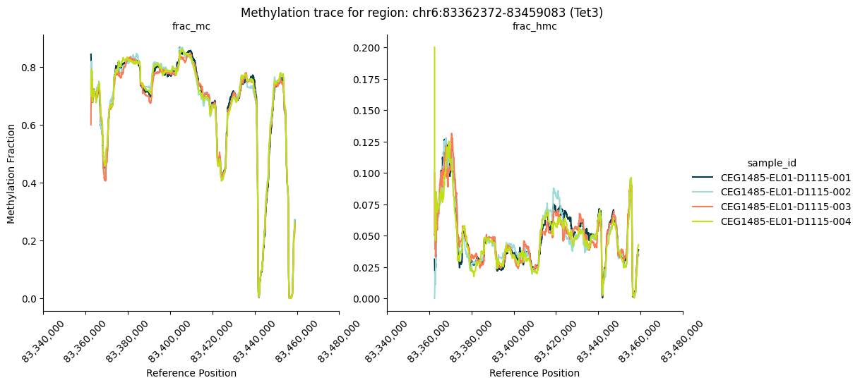
"tet3_slice": ds["chr6:83362372-83459083"],
}
Generate methylation trace plots#
Using the slices of data defined above we can easily generate methylation trace plots to show how different samples in the dataset vary in their methylation fractions across specified genomic regions. To do so we make use of the plot_methylation_trace() method from ContigDataset. This method computes methylation fractions from the specified num_* variables (specified with the numerators argument) against a num_total* variable and will return a seaborn.relplot plot.
Please note: this method is meant for plotting small regions covering up to a maximum of 200,000 CpGs.
sliced_data['slice_1'].plot_methylation_trace(
    numerators=["num_mc", "num_hmc"],
    denominator="num_total_c",
    min_coverage=10,
    title="Methylation trace for region: chr10:44391523-44392442",
)
<seaborn.axisgrid.FacetGrid at 0x33c484190>
sliced_data['tet1_slice'].plot_methylation_trace(
    numerators=["num_mc", "num_hmc"],
    denominator="num_total_c",
    min_coverage=10,
    title="Methylation trace for region: chr10:62804569-62908995 (Tet1)",
)
<seaborn.axisgrid.FacetGrid at 0x33c571390>
sliced_data['tet3_slice'].plot_methylation_trace(
    numerators=["num_mc", "num_hmc"],
    denominator="num_total_c",
    min_coverage=10,
    title="Methylation trace for region: chr6:83362372-83459083 (Tet3)",
)
<seaborn.axisgrid.FacetGrid at 0x33cb40b90>